Infimal convolution-based regularization for SPECT reconstruction

Abstract

Purpose: Total variation (TV) regularization is efficient in suppressing noise, but is known to suffer from staircase artifacts. The goal of this work was to develop a regularization method using the infimal convolution of the first- and the second-order derivatives to reduce or even prevent staircase artifacts in the reconstructed images, and to investigate if the advantage in noise suppression by this TV-type regularization can be translated into dose reduction.

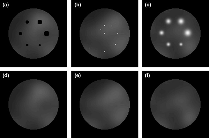
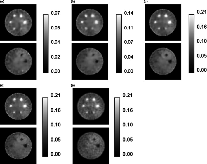
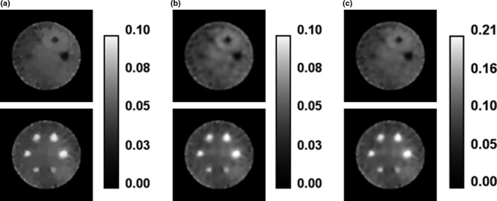
Methods: In the present work, we introduce the infimal convolution of the first- and the second-order total variation (ICTV) as the regularization term in penalized maximum likelihood reconstruction. The preconditioned alternating projection algorithm (PAPA), previously developed by the authors of this article, was employed to produce the reconstruction. Using Monte Carlo-simulated data, we evaluate noise properties and lesion detectability in the reconstructed images and compare the results with conventional total variation (TV) and clinical EM-based methods with Gaussian post filter (GPF-EM). We also evaluate the quality of ICTV regularized images obtained for lower photon number data, compared with clinically used photon number, to verify the feasibility of radiation-dose reduction to patients by use of the ICTV reconstruction method.

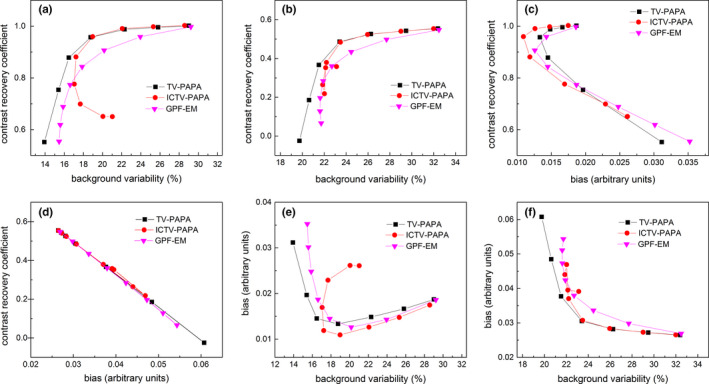
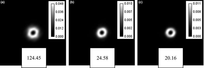
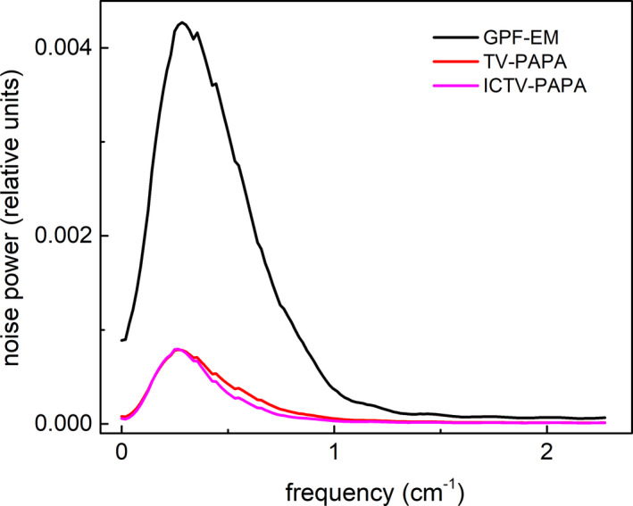
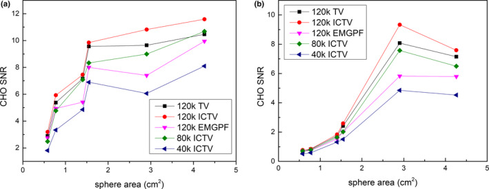
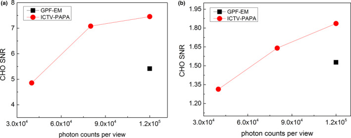
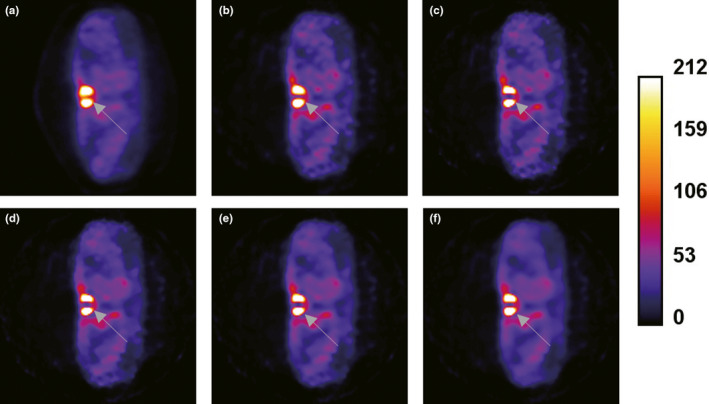
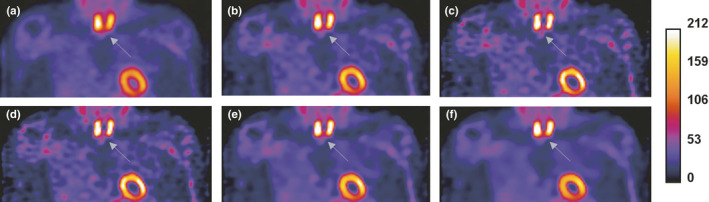
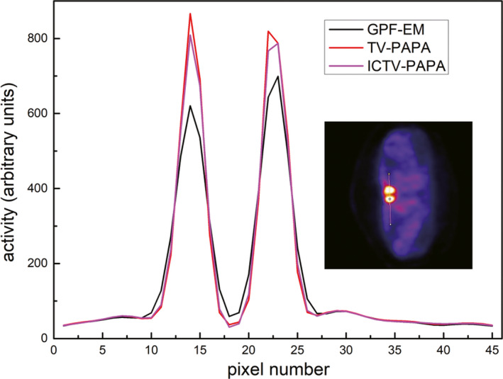
Results: By comparison with GPF-EM reconstructed images, we have found that the ICTV-PAPA method can achieve a lower background variability level while maintaining the same level of contrast. Images reconstructed by the ICTV-PAPA method with 80,000 counts per view exhibit even higher channelized Hotelling observer (CHO) signal-to-noise ratio (SNR), as compared to images reconstructed by the GPF-EM method with 120,000 counts per view.

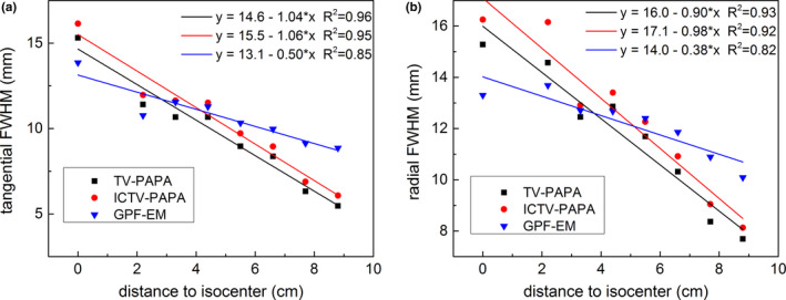
Conclusions: In contrast to the TV-PAPA method, the ICTV-PAPA reconstruction method avoids substantial staircase artifacts, while producing reconstructed images with higher CHO SNR and comparable local spatial resolution. Simulation studies indicate that a 33% dose reduction is feasible by switching to the ICTV-PAPA method, compared with the GPF-EM clinical standard.

Keywords: SPECT reconstruction; fixed-point proximity methods; infimal convolution; noise suppression; penalized maximum likelihood optimization total variation regularization; staircase artifact.

Figure 1

Transaxial cross‐sections of a phantom with: (a) six cold (no activity) piecewise constant spheres with radii of 4, 5, 6, 7, 8, and 9 mm, (b) eight point sources with maximum‐activity‐to‐mean‐background ratio of 100:1 at different radial distances from the central axis of the phantom, (c) six hot Gaussian blobs with radii (FWHM) of 4, 5, 6, 7, 8, and 9 mm with maximum‐activity‐to‐mean‐background ratio of 3:1 and (d–f) reference phantom containing warm Gaussian blobs only. Both phantoms were of the size 128 × 128 × 128 voxels, with voxel size set to 2.2 × 2.2 × 2.2 mm³.

Figure 2

Transaxial cross‐sections of images for Monte Carlo‐simulated SPECT data for phantom shown in Fig. 1, reconstructed by: (a) the ICTV‐PAPA method for 40 kc/view data, λ ₁  = 0.4, λ ₂  = 0.4; (b) the ICTV‐PAPA method for 80 kc/view data, λ ₁  = 0.3, λ ₂  = 0.3; (c) the ICTV‐PAPA method for 120 kc/view data, λ ₁  = 0.2, λ ₂  = 0.2; (d) the TV‐PAPA method for 120 kc/view data, λ = 0.2; and (e) the GPF‐MLEM method using 120 kc/view data, FWHM = 7.3 mm. For all images, reconstructions were stopped at 100 iterations. Left column: hot spheres with Gaussian activity distribution (see text). Right column: cold spheres with zero activity.

Figure 3

Components of the ICTV‐PAPA‐reconstructed images obtained at 100 iterations for simulated SPECT data with 120 kc/view, λ ₁  = 0.2, and λ ₂  = 0.2: (a) f ₁ component, (b) f ₂ component, and (c) final combined image (f = f ₁  + f ₂ ). Top row: cold spheres with zero activity. Bottom row: hot spheres with Gaussian activity distribution (see Fig. 1 and text).

Figure 4

(a) Mean CRC vs. background variability for hot spheres; (b) Mean CRC vs. background variability for cold spheres; (c) Mean CRC vs. bias for hot spheres; (d) Mean CRC vs. bias for cold spheres; (e) Bias vs. background variability for hot spheres; (f) Bias vs. background variability for cold spheres. Each point on the curves was calculated for penalty parameters selected in the 0.01–200 range for TV‐based algorithms and Gaussian post‐filter radii in the 1.1–7.1 mm range for GPF‐EM. Only the four largest spheres were considered among cold spheres. The true background spatial variability for selected ROIs is 17.6% for the background in the cross‐section with hot spheres and 22.7% for the cross‐section with cold spheres due to the lumpy background. [Color figure can be viewed at wileyonlinelibrary.com]

Figure 5

Local noise power spectra (LNPS) obtained for the central location of small ROI: (a) the GPF‐EM method; (b) the TV‐PAPA method; and (c) the ICTV‐PAPA method all obtained for simulated SPECT data with 120 kc/view. Noise variance values of the selected ROI and penalty parameters are displayed at the bottom of each image.

Figure 6

Average radial profiles for local noise power spectra shown in Fig. 5. The profiles were obtained by averaging the data every 10°. [Color figure can be viewed at wileyonlinelibrary.com]

Figure 7

CHO detectability indices of (a) hot; and (b) cold spheres vs. cross‐sectional area of the spheres and vs. the number of counts per view in the simulated SPECT data. The ICTV‐PAPA method for 40 kc/view data, λ ₁  = 0.4, λ ₂  = 0.4; the ICTV‐PAPA method for 80 kc/view data, λ ₁  = 0.3, λ ₂  = 0.3; the ICTV‐PAPA method for 120 kc/view data, λ ₁  = 0.2, λ ₂  = 0.2; the TV‐PAPA method for 120 kc/view data, λ = 0.2; and the GPF‐MLEM method using 120 kc/view data, FWHM = 7.3 mm. The reconstructions were stopped at 100 iterations. The solid lines connecting the data points are provided as a visual guide only. [Color figure can be viewed at wileyonlinelibrary.com]

Figure 8

CHO detectability indices estimated (solid circles) for the fourth largest sphere (1.4 cm² cross‐sectional area) for images reconstructed with three photon levels (40, 80, and 120 kc/view) using the ICTV‐PAPA method and the GPF‐EM method (solid squares) at 120 kc/view level. The solid lines connecting the data points are provided as a visual guide. [Color figure can be viewed at wileyonlinelibrary.com]

Figure 9

(a) Radial full width at half maximum (FWHM) and (b) tangential FWHM of transaxial local point spread function (LPSF) as a function of radial positions of point sources. The SPECT data were simulated for 120 kc/view. Reconstructions were performed with the following penalty parameters: the ICTV‐PAPA method for 40 kc/view data, λ ₁  = 0.4, λ ₂  = 0.4; the ICTV‐PAPA method for 80 kc/view data, λ ₁  = 0.3, λ ₂  = 0.3; the ICTV‐PAPA method for 120 kc/view data, λ ₁  = 0.2, λ ₂  = 0.2; the TV‐PAPA method for 120 kc/view data, λ = 0.2; and the GPF‐EM method using 120 kc/view data, FWHM = 7.3 mm. Reconstructions were stopped at 100 iterations. The solid lines are linear regression fits. [Color figure can be viewed at wileyonlinelibrary.com]

Figure 10

Transaxial views of reconstructed images obtained for clinical Tc‐99 m Sestamibi SPECT parathyroid, late‐phase study: the clinical Hermes HOSEM method (a); the GPF‐EM method (b); the TV (c, d); and ICTV‐PAPA (e, f) methods, each with two sets of penalty parameters. [Color figure can be viewed at wileyonlinelibrary.com]

Figure 11

Coronal views of reconstructed images obtained for clinical Tc‐99 m Sestamibi SPECT parathyroid late‐phase study: the clinical Hermes HOSEM method (a); the GPF‐EM method (b); the TV (c, d); and ICTV‐PAPA (e, f) methods, each with two sets of penalty parameters. [Color figure can be viewed at wileyonlinelibrary.com]

Figure 12

One‐channel‐wide line profiles through reconstructed transaxial images of clinical Tc‐99 m Sestamibi parathyroid scan image shown in Fig. 10. The location of the profile is shown in the inset. Penalty weights were set as: the TV‐PAPA method: λ = 2, the ICTV‐PAPA method: λ ₁ = 2, λ ₂ = 2. [Color figure can be viewed at wileyonlinelibrary.com]

References

1. Bertero M, Boccacci P. Introduction to Inverse Problems in Imaging. Boca Roton, FL: CRC Press; 1998.
1. Geman S, Geman D. Stochastic relaxation, gibbs distributions, and the bayesian restoration of images. IEEE Trans Pattern Anal Mach Intell. 1984;6:721–741. - PubMed
1. Geman S, MacClure D. Bayesian Image Analysis: An Application to Single Photon Emission Tomography. Alexandria, VA: American Statistical Association; 1985.
1. Rudin LI, Osher S, Fatemi E. Nonlinear total variation based noise removal algorithms. Physica D. 1992;60:259–268.
1. Panin VY, Zeng GL, Gullberg GT. Total variation regulated EM algorithm [SPECT reconstruction]. IEEE Trans Nucl Scie. 1999;46:2202–2210.