A topographic mechanism for arcing of dryland vegetation bands

Abstract

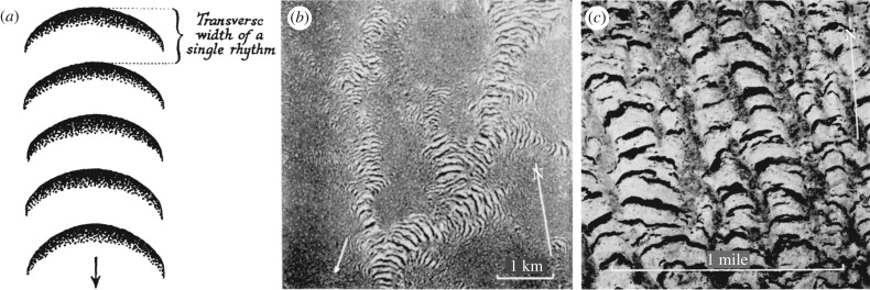
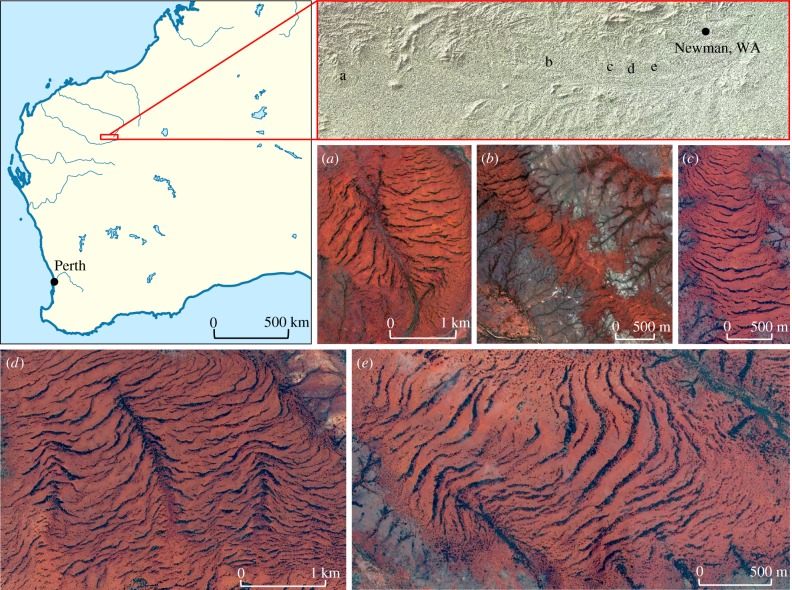
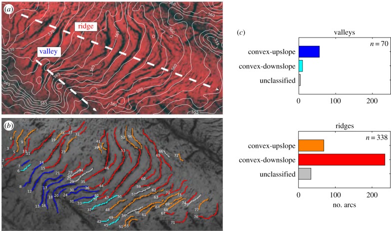
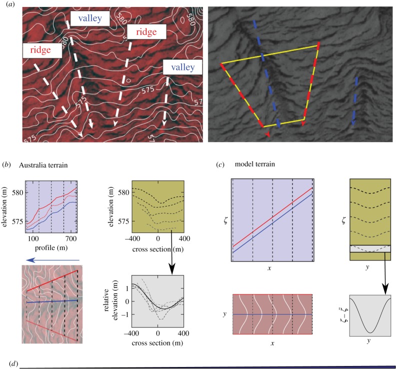
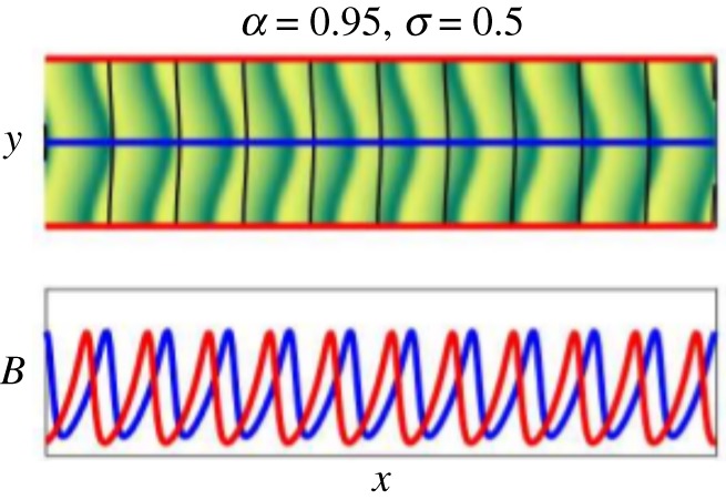
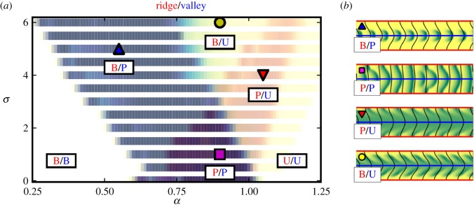
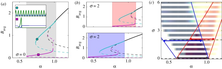
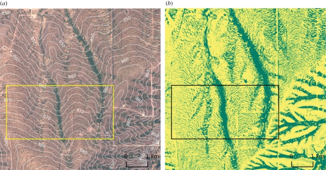
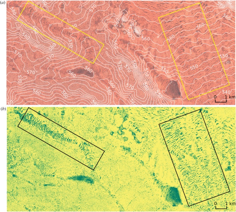
Banded patterns consisting of alternating bare soil and dense vegetation have been observed in water-limited ecosystems across the globe, often appearing along gently sloped terrain with the stripes aligned transverse to the elevation gradient. In many cases, these vegetation bands are arced, with field observations suggesting a link between the orientation of arcing relative to the grade and the curvature of the underlying terrain. We modify the water transport in the Klausmeier model of water-biomass interactions, originally posed on a uniform hillslope, to qualitatively capture the influence of terrain curvature on the vegetation patterns. Numerical simulations of this modified model indicate that the vegetation bands arc convex-downslope when growing on top of a ridge, and convex-upslope when growing in a valley. This behaviour is consistent with observations from remote sensing data that we present here. Model simulations show further that whether bands grow on ridges, valleys or both depends on the precipitation level. A survey of three banded vegetation sites, each with a different aridity level, indicates qualitatively similar behaviour.

Keywords: dryland ecology; early warning signs; pattern formation; reaction–advection–diffusion; spatial ecology; vegetation patterns.

Figure 1.

Aerial photographs of vegetation patterns found in the Horn of Africa alongside (a) a schematic adapted from [5] showing typical orientation relative the topography. The vegetation bands are aligned transverse to the slope and arc convex-upslope. The banded patterns in image (b), adapted from [5], appear within topographic depressions and the darker unpatterned regions of image (c), adapted from [6], are reported to be slightly elevated relative to the vegetation arcs. Arrows in (a) and (b) indicate downhill direction.

Figure 2.

Five sites displaying banded vegetation patterns in the Western Creek Basin southwest of Newman, Australia (−23.5° N, 119.5° E), alongside a map indicating the relative location of each site. The Sentinel-2A images [28] were taken near the end of the Australian wet season, see scale bars for relative sizes. Map derived from image available via Wikimedia Commons. (Online version in colour.)

Figure 3.

(a) An example site with elevation contours (solid white) and manually identified ridge/valley lines (dashed white, with arrows indicating the downhill direction). (b) The manually identified arcs are coloured by the classification: convex-upslope in valley (blue), convex-downslope in valley (cyan), convex-upslope on ridge (orange) and convex-downslope on ridge (red). (c) Bar chart of the 408 vegetation arcs from the five sites of figure 2 that have been manually identified and classified as appearing in either a valley or on a ridge and as convex-upslope or convex-downslope. (Online version in colour.)

Figure 4.

(a) The left image shows elevation contours (solid white) on a section of the patterned site in figure 2d. A few approximate ridge and valley lines (white dashed) are shown with arrows pointing downhill. The yellow trapezoid in the right greyscale image indicates a typical topographic structure consisting of a valley aligned along the grade surrounded by two ridges. (b) Elevation contours for the trapezoid region in (a) are shown together with their profiles along the grade (above) and along cross sections transverse to the grade (right). A fourth-order polynomial fit (solid black) is shown for the elevation relative to the mean of the cross sections (dotted grey). Note that the profile distance is taken to be distance along the valley line and the associated ridge elevations are found by orthogonal projection. (c) Model topography given by equation (1.5) with v = 10, σ = 5, L_x = 100 and L_y = 50. Elevation contours along with cross sections show the height of ridge (red) and valley (blue) relative to the change in elevation that results from uniform slope along x. Note that the scale for elevation in (a) and (b) is greatly exaggerated relative to the x- and y-dimensions. (d) For reference, the triangle at the bottom is drawn to scale with a 0.6% grade corresponding to the mean of the example shown in (b). (Online version in colour.)

Figure 5.

Upper frame shows biomass field on the full two-dimensional domain at t = 1000 with the modestly curved elevation contours (black) superimposed. Green (yellow) on the colour scale represents high (low) biomass values. While the vegetation bands are more significantly arced than the elevation contours, the direction of curvature consistently matches across the domain for both. The lower frame shows one-dimensional profiles of the biomass along ridge (red) and valley (blue) lines. Periodic domain: L_x = 200, L_y = 50. Parameters: a = 0.95, m = 0.45, v = 10, k₀ = 2π/L_y. (Online version in colour.)

Figure 6.

(a) Maximum amplitude of patterns on ridges and valleys in (a, σ)-plane when precipitation a is decreased and then increased for fixed channel aspect σ. Yellow indicates small amplitude while red (blue) indicates large amplitude on ridge (valley) and purple indicates large amplitude on ridge and in valley. Each region is labelled by ridge/valley state as bare soil (B), patterned (P) or uniformly vegetated (U). (b) Biomass from simulations initialized with uniform vegetation and parameters associated with the labelled points the (a, σ)-plane are shown for t = 1000. Parameters: m = 0.45, v = 10, k₀ = 2π/50. (Online version in colour.)

Figure 7.

(a) Bifurcation diagram of one-dimensional Klausmeier model given by equations (3.2) and (3.3) showing uniform vegetation state (black) and two of the family of travelling wave solutions that bifurcate from the upper branch of this state: the Turing–Hopf branch (cyan) and the branch corresponding to a single pulse of biomass on the domain (magenta). Stable (unstable) solutions are indicated by thick solid (thin dashed) lines and at least one solution from this family is stable within the interval of a shaded in grey. (b) Bifurcation diagrams for the model with effective water loss rate corresponding to the ridge and valley for σ = 2 are compared to the model with σ = 0. The region shaded red (blue) indicates the existence of stable travelling wave solutions for the model associated with the ridge (valley). (c) Boundaries of predicted regions of existence for ridge (red) and valley (blue) patterns based on one-dimensional models. The results are superimposed on the two-dimensional simulations shown in figure 6a for comparison. These numerical continuation results were computed with AUTO [33], see §3.3 for more details. Parameters: v = 10, m = 0.45, k₀ = 2π/50, L_x = 200. (Online version in colour.)

Figure 8.

Satellite image (a) and maximum NDVI (b) of a 7 km by 7 km region northwest of Ft Stockton, TX, USA that exhibits vegetation bands on the northwest face (upper left) of a hill. The boxed region shows a 5 km by 2.5 km area with a series of ridges and valleys aligned along the slope. The broad ridge on the right of the box is about 2 km across, measured between the two uniform vegetation valleys, and has a valley-to-ridge elevation gain of about 5 m. Four smaller valleys can also be observed with characteristic transverse width of 300–400 m and transverse elevation changes less than a metre. The mean slope along this northwest face is about 0.6% (approx. 40 m over 6.6 km). The southeast face (lower right) is steeper, with an average grade of about 0.75%, and the vegetation is organized into a network of channels with ridge-to-ridge spacing ranging from 300 m to 800 m and valley-to-ridge depth ranging from 1 m for the narrower channels to 6 m for the larger central channels that the narrower channels feed into. The satellite imagery comes from Sentinel 2 [28] while the elevation comes from the US National Elevation Dataset [38]. The RGB image was chosen from the least cloudy day between October 2016 and May 2017. High (low) values for maximum NDVI at each pixel over the 2 year period May 2015 to May 2017 are shown with green (yellow). (Online version in colour.)

Figure 9.

Satellite image (a) and maximum NDVI (b) of a 21 km by 10 km region of Ethiopia located just east of the site shown in figure 1b. Two areas within the image are highlighted by boxes. The left is a channel aligned along a overall slope of about 0.2% grade with an approximate ridge-to-ridge distance of 3 km. The vegetation pattern, with bands arcing convex-upslope, appears within a 2 km region surrounding the valley line where the transverse elevation has a 2 m variation from minimum to maximum. The region highlighted on the right is within a broad, relatively flat valley with an overall 0.3% grade and transverse variations of less than 1 m across the 4 km width of the box. The satellite imagery comes from Sentinel 2 [28] while the elevation data are ALOS [39] with spectral smoothing [40]. The RGB image is of the least cloudy day between October 2016 and May 2017 and the NVDI shows maximum value at each pixel over the same time period. (Online version in colour.)

References

1. Borgogno F, D'Odorico P, Laio F, Ridolfi L. 2009. Mathematical models of vegetation pattern formation in ecohydrology. Rev. Geophys. 47, 195 (10.1029/2007RG000256) - DOI
1. Deblauwe V, Barbier N, Couteron P, Lejeune O, Bogaert J. 2008. The global biogeography of semi-arid periodic vegetation patterns. Global Ecol. Biogeogr. 17, 715–723. (10.1111/j.1466-8238.2008.00413.x) - DOI
1. Rietkerk M, Dekker SC, de Ruiter PC, van de Koppel J. 2004. Self-organized patchiness and catastrophic shifts in ecosystems. Science 305, 1926–1929. (10.1126/science.1101867) - DOI - PubMed
1. Dakos V, Kéfi S, Rietkerk M, Van Nes EH, Scheffer M. 2011. Slowing down in spatially patterned ecosystems at the brink of collapse. Am. Nat. 177, E153–E166. (10.1086/659945) - DOI - PubMed
1. Macfadyen WA. 1950. Vegetation patterns in the semi-desert plains of British Somaliland. Geogr. J. 116, 199–211. (10.2307/1789384) - DOI
Publication types
LinkOut - more resources