State observation and sensor selection for nonlinear networks

Abstract

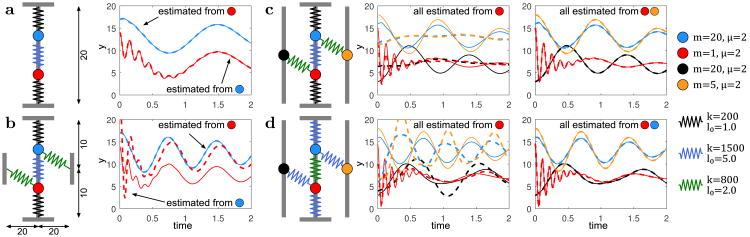
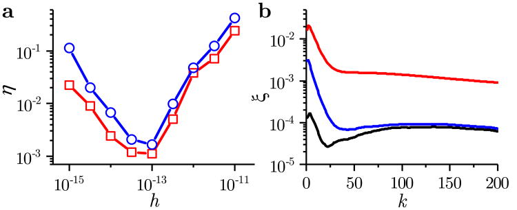
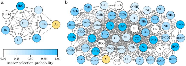
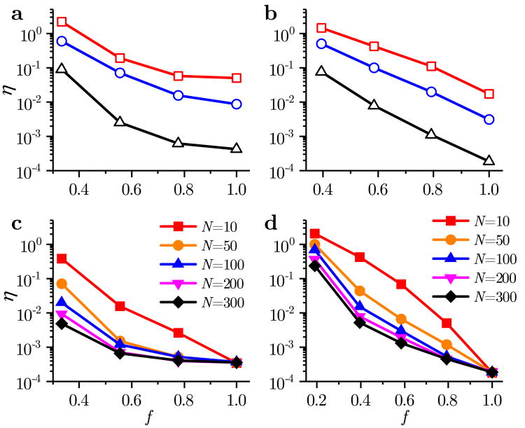
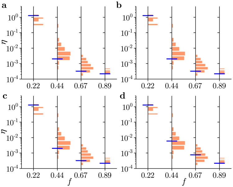
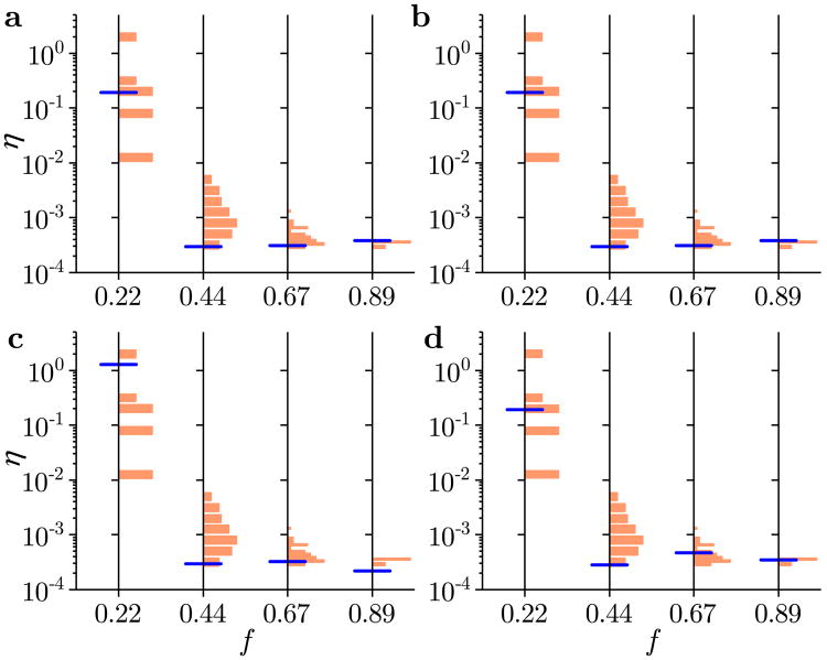
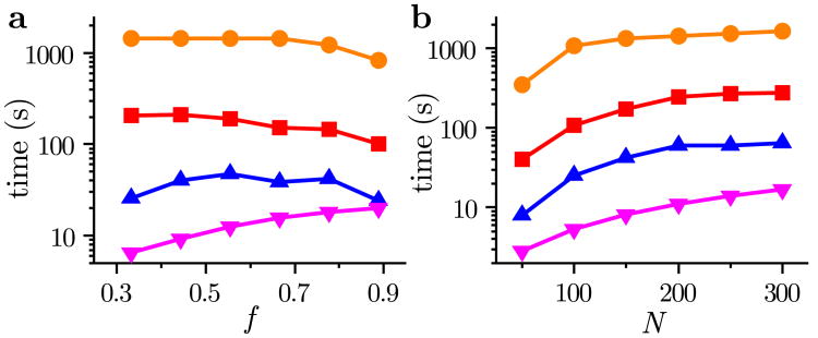
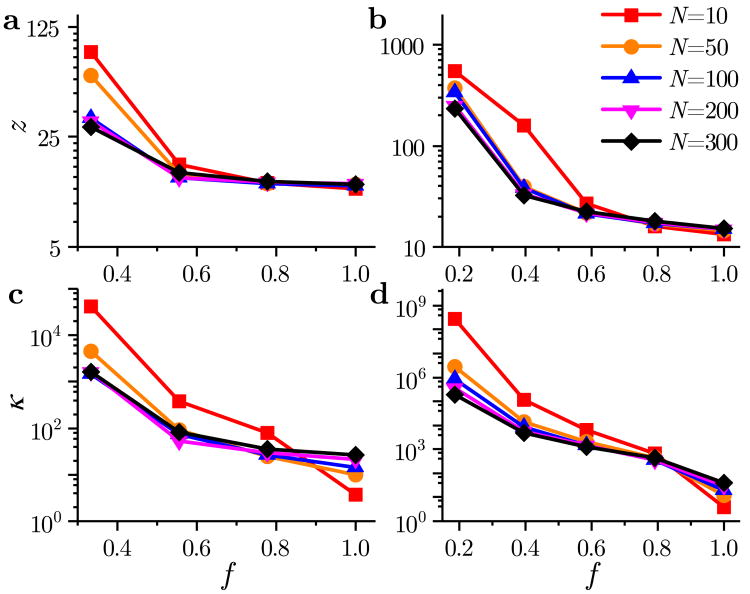
A large variety of dynamical systems, such as chemical and biomolecular systems, can be seen as networks of nonlinear entities. Prediction, control, and identification of such nonlinear networks require knowledge of the state of the system. However, network states are usually unknown, and only a fraction of the state variables are directly measurable. The observability problem concerns reconstructing the network state from this limited information. Here, we propose a general optimization-based approach for observing the states of nonlinear networks and for optimally selecting the observed variables. Our results reveal several fundamental limitations in network observability, such as the trade-off between the fraction of observed variables and the observation length on one side, and the estimation error on the other side. We also show that, owing to the crucial role played by the dynamics, purely graph-theoretic observability approaches cannot provide conclusions about one's practical ability to estimate the states. We demonstrate the effectiveness of our methods by finding the key components in biological and combustion reaction networks from which we determine the full system state. Our results can lead to the design of novel sensing principles that can greatly advance prediction and control of the dynamics of such networks.

Keywords: complex networks; observability; sensor selection; state and parameter estimation.

Figure 1

State estimation in spring-mass networks. Networks of (a) two masses subject to linear forces, (b) two masses subject to nonlinear forces, and (c, d) four masses subject to nonlinear forces. In each case, the point masses are restricted to move vertically and the forces (including the nonlinear ones) are emulated by linear springs in the plane. The spring constants k, rest lengths l₀, friction coefficients μ, and masses m are color-coded (legend on the right); the dimensions of the systems are marked on the figure (the dimensions in c and d are the same as in b). The initial states (position and velocity) of each mass are estimated only from the direct observation of the position of the subset of masses marked on the plots. The plots compare the true trajectories over time (solid lines) and those calculated from estimated initial states (dashed lines), color-coded as the masses. In a (linear case), estimation is successful from the observations of either mass, whereas in b (nonlinear case), estimation is successful only if the smaller mass is observed. In c and d (larger networks), estimation is only successful if at least two masses are observed; comparison between c and d further shows that the optimal sensor placement (directly observed masses) depends not only on the OID but also on the dynamical parameters. Note that this is the case even though each network has as single (root) SCC.

Figure 2

Accuracy of the discretization methods. (a) Estimation error η as a function of the discretization step size h, for the H₂/O₂ (squares) and GRI-Mech 3.0 (circles) networks, using the IRK model. (b) Comparison of the time-dependent error ${\xi }_k={\Vert {\mathbf{x}}_k-{\mathbf{x}}_k^{\ast }\Vert }_2/{\Vert {\mathbf{x}}_k^{\ast }\Vert }_2$ for each step k, where ${\mathbf{x}}_k\in {\mathbb{R}}_{\ge 0}^n$ is computed using the BE (red line), TI (blue line), and IRK (black line) discretization methods. This comparison is for the H₂/O₂ network, with N = 200, h = 10⁻¹³, and ${\mathbf{x}}_k^{\ast }$ computed using ode15s. In both panels, the results are averaged over 100 realizations of random initial conditions, as defined in equation (23).

Figure 3

OIDs and sensor selection probabilities for combustion networks. OIDs of the (a) H₂/O₂ network and (b) GRI-Mech 3.0 network, where self-loops are omitted for clarity. Color-coded is the probability of selecting the node using the optimal sensor selection method (see text). Each network consists of two SCCs, one formed by Ar (always taken as a sensor) and the other by the remaining nodes. The data were computed using the IRK model for N = 200 and h = 10⁻¹³.

Figure 4

Estimation error η as function of the sensor fraction f and observation length N. Results for the (a, c) H₂/O₂ network and (b, d) GRI-Mech 3.0 network. Panels a and b compare the three models (Δ-IRK, ○-TI, and □-BE) for N = 50, whereas panels c and d compare different N for the IRK model. Each data point is an average over 100 realizations of the random sensor placement and initial guesses of the solution in the GRI-Mech 3.0 network and over all possible placement configurations in the H₂/O₂ network. The discretization step was h = 10⁻¹³ in all simulations.

Figure 5

Optimal sensor selection for the combustion networks. Estimation error η for the (a) H₂/O₂ network and (b) GRI-Mech 3.0 network. For each network and sensor fraction f, the histogram presents η for an exhaustive calculation in panel a and for 100 realizations of the random sensor placement in panel b. The blue line marks the estimation error for the calculated optimal sensor selection. The results are generated using the IRK model for N = 200 and h = 10⁻¹³.

Figure 6

OIDs and sensor selection probabilities for biological networks. Same as in Fig. 3 for the (a) CD network and (b) SS network. Yellow indicates single-node SCCs, whereas the remaining nodes belong to a giant SCC. Sensors are placed on the yellow nodes a priori, which are then excluded from the optimal sensor selection. The data were computed using the IRK model for N = 100 and h = 0.02 in panel a, and for N = 100 and h = 0.05 in panel b.

Figure 7

Estimation error η for the (a) CD network and (b) SS network as a function of the observation horizon and sensor fraction. The results are generated for the IRK model with h = 0.02 in panel a and h = 0.05 in panel b. The results are averages over 100 realizations of the random sensor selections and random initial conditions.

Figure 8

Optimal sensor selection for the biological networks. Estimation error η for the (a) CD network and (b) SS network. For each network and sensor fraction f, the histogram presents η for 100 realizations of the random sensor placement. The blue line marks the estimation error for the calculated optimal sensor selection; the red line indicates the corresponding result when information about the OID is ignored. The results are generated using the IRK model for N = 100 and h = 0.02 in panel a, and for N = 100 and h = 0.05 in panel b.

Figure 9

Four methods for sensor selection validated and compared on the H₂/O₂ network for short observation length. Estimation error η for (a) Method 1, (b) Method 2, (c) Method 3, and (d) Method 4. The histograms correspond to the estimation errors for all possible combinations of the sensor nodes. The network is sufficiently small that exhaustive calculation of all combinations is possible in this case. The blue line represents the estimation error for the optimal sensor selection. The results are obtained for N = 50, h = 10⁻¹³, and the IRK model.

Figure 10

Same as in Fig. 9 for the longer observation time of N = 200.

Figure 11

Computational time for sensor selection as a function of (a) the fraction of observed nodes f and (b) the observation horizon N. The various curves correspond to Method 1 (■), Method 2 (●), Method 3 (▴), and Method 4 (▾), applied to the GRI-Mech 3.0 network. Results are averaged over 10 random initial guesses for the selected sensors, using the IRK model and h = 10⁻¹³, for N = 200 in panel a and f = 0.5 in panel b.

Figure 12

Convergence and condition numbers of Jacobians of the nonlinear least-squares problem defined by equation (10). (a, b) Number of iterations z to compute the estimate as a function of the sensor fraction f and the observation horizon N. (c, d) Condition number κ of the Jacobian matrix at the final estimate. Panels a and c correspond to the H₂/O₂ network, panels b and d correspond to the GRI-Mech 3.0 network. The parameters are the same as the ones used in Fig. 4, panels c and d.

Figure 13

Computational complexity of solving the nonlinear least-squares problem defined by equation (10). The computational complexity is shown for the H₂/O₂ (■) and GRI-Mech 3.0 (●) networks as a function of (a) the fraction of the observed nodes f and of (b) the observation horizon N. In panel a the results correspond to an average of 100 samples of randomly selected sensors and N = 200, whereas in panel b the results correspond to f = 0.6. In both panels, the results are obtained for the IRK model and h = 10⁻¹³.

References

1. Camacho EF, Alba CB. Model Predictive Control. London: Sprinver-Verlag; 2007.
1. Khalil HK. Nonlinear Systems. Upper Saddle River, NJ: Prentice Hall; 2002.
1. Whalen AJ, Brennan SN, Sauer TD, Schiff SJ. Observability and controllability of nonlinear networks: the role of symmetry. Phys Rev X. 2015;5:011005. - PMC - PubMed
1. Yan G, et al. Spectrum of controlling and observing complex networks. Nat Phys. 2015;11:779–786.
1. Lin F, Fardad M, Jovanović MR. Design of optimal sparse feedback gains via the alternating direction method of multipliers. IEEE Trans Autom Control. 2013;58:2426–2431.
LinkOut - more resources