Modeling large fluctuations of thousands of clones during hematopoiesis: The role of stem cell self-renewal and bursty progenitor dynamics in rhesus macaque

Abstract

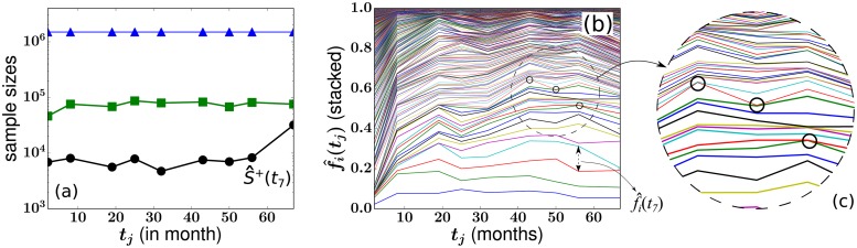
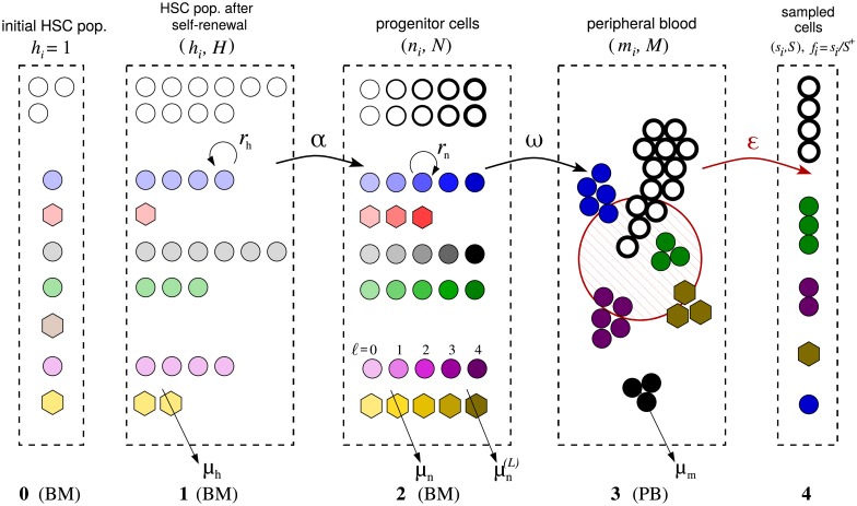
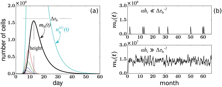
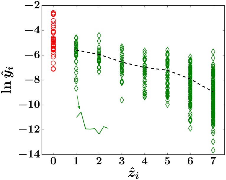
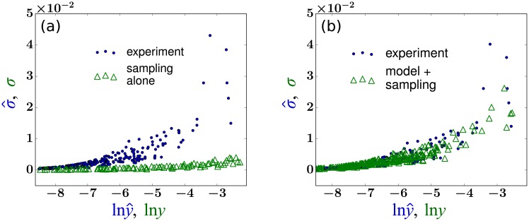
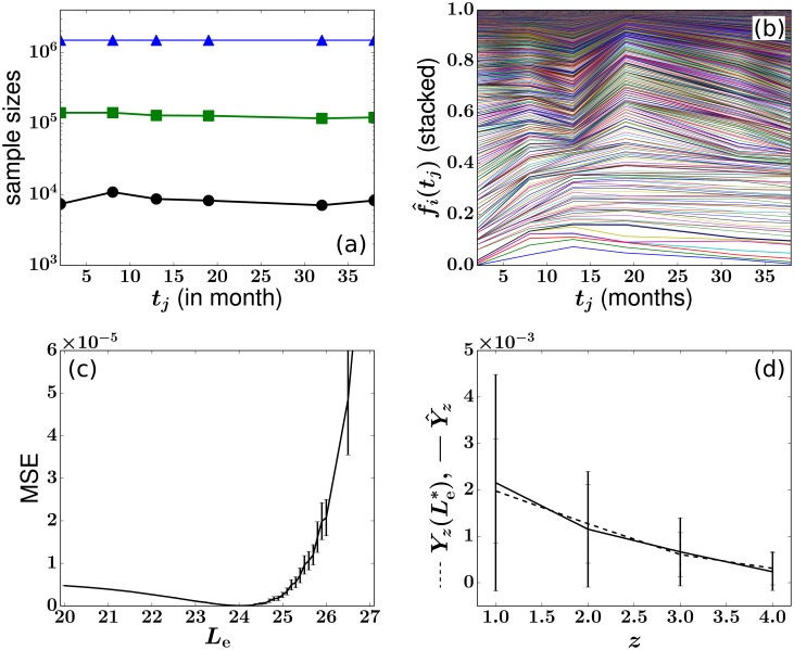
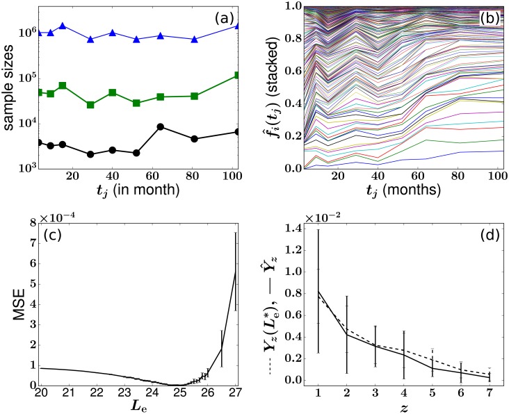
In a recent clone-tracking experiment, millions of uniquely tagged hematopoietic stem cells (HSCs) and progenitor cells were autologously transplanted into rhesus macaques and peripheral blood containing thousands of tags were sampled and sequenced over 14 years to quantify the abundance of hundreds to thousands of tags or "clones." Two major puzzles of the data have been observed: consistent differences and massive temporal fluctuations of clone populations. The large sample-to-sample variability can lead clones to occasionally go "extinct" but "resurrect" themselves in subsequent samples. Although heterogeneity in HSC differentiation rates, potentially due to tagging, and random sampling of the animals' blood and cellular demographic stochasticity might be invoked to explain these features, we show that random sampling cannot explain the magnitude of the temporal fluctuations. Moreover, we show through simpler neutral mechanistic and statistical models of hematopoiesis of tagged cells that a broad distribution in clone sizes can arise from stochastic HSC self-renewal instead of tag-induced heterogeneity. The very large clone population fluctuations that often lead to extinctions and resurrections can be naturally explained by a generation-limited proliferation constraint on the progenitor cells. This constraint leads to bursty cell population dynamics underlying the large temporal fluctuations. We analyzed experimental clone abundance data using a new statistic that counts clonal disappearances and provided least-squares estimates of two key model parameters in our model, the total HSC differentiation rate and the maximum number of progenitor-cell divisions.

Fig 1. Blood sample data from animal RQ5427 [13].

(a) The total numbers of sampled granulocytes (blue triangles), EGFP+ granulocytes (green squares), and the subset of EGFP+ granulocytes that were properly tagged and quantifiable were extracted for PCR amplification and analysis (black circles). This last population defined by ${\widehat{S}}^{+}\left(t_j\right)$ is used to normalize clone cell counts. We excluded the first sample at month 2 in our subsequent analysis so, for example, the sample at month 56 is labeled the 7th sample. There were 536 clones detected at least once across the eight samples taken over 67 months comprising an average fraction 0.052 of all granulocytes. The abundances of granulocyte clones are shown in (b). The relative abundance ${\widehat{f}}_i\left(t_j\right)$ of granulocytes from the i^th clone measured at month t_j is indicated by the vertical distances between two adjacent curves. The relative abundances of individual clones feature large fluctuations over time. “Extinctions” followed by subsequent “resurrections,” were constantly seen in certain clones as indicated by the black circles in (b) and in the inset (c).

Fig 2. Schematic of a neutral multi-stage or multi-compartment hematopoiesis model.

BM and PB refer to bone marrow and peripheral blood, respectively. Cells of the same clone have the same color. White circles represent untagged cells which were not counted in the analysis. Stages 0, 1, and 2 describe cell dynamics that occur mainly in the bone marrow. Stage 1 describes HSC clones (C_h = 6 in this example) after self-renewal that starts shortly after transplantation with rate r_h. After self-renewal, the relatively stable HSC population (H⁺ = 20 in this example) shifts its emphasis to differentiation (with per-cell differentiation rate α). Larger clones in Stage 1 (e.g., the circular blue clone, h_blue = 4) will have a larger total differentiation rate αh_blue while smaller clones (e.g., the red hexagonal clone, h_red = 1) will have smaller αh_red. The processes of progenitor-cell proliferation (with rate r_n) and maturation (with rate ω) in Compartments 2 and 3 are considered deterministic because of the large numbers of cells involved. The darker-colored symbols correspond to cells of later generations. For illustration, the maximum number of progenitor-cell generations allowed is taken to be L = 4. Compartment 4 represents a small sampled fraction (ε(t_j) ≈ 2.8 × 10⁻⁵ − 2 × 10⁻⁴) of Compartment 3, the entire peripheral blood of the animal. In the example pictured above, C_s = 4. Such small samples can lead to considerable sampling noise but is not the key driver of sample-to-sample variability.

Fig 3

(a) A burst of cells is triggered by a single HSC differentiation event at time t = 0. A plot of representative solutions to Eqs (10) and (11) for r_n = 2.5, L = 24, ${\mu }_{\mathrm{n}}={\mu }_{\mathrm{n}}^{\left(L\right)}=0$, μ_m = 1, $A_{\text{ss}}^{+}=14.7$, and ω = 0.16. Curves of different colors represent $n_{\mathrm{b}}^{\left(\ell \right)}\left(t\right)$, the progenitor cell population within each generation ℓ = 0, 1, 2, …, L, and m_b(t), the number of mature granulocytes associated with the differentiation burst. All populations rise and fall. (b) Realizations of peripheral blood (PB) populations in a single clone arising from multiple successive differentiation events. The fluctuating populations are generated by adding together m_b(t) associated with each differentiation event. Time series resulting from small (h_i/H⁺ = 0.0003) and large (h_i/H⁺ = 0.03) HSC clones are shown. Small clones are characterized by separated bursts of cells, after which the clone vanishes for a relatively long period of time. The number of mature peripheral blood cells of large clones reaches a relatively constant level and almost never vanishes.

Fig 4. Scatterplot of clone trajectories of animal RQ5427 displayed in terms of ln y^i, the log mean abundance of clone i, and z^i, the number of samples in which clone i is undetected.

The trajectory of each clone i is represented by a symbol located at a coordinate determined by its value of ln ${\widehat{y}}_i$ and ${\widehat{z}}_i$. A trajectory of a clone that exhibits one absence within months 8 − 67 is shown in the inset. The first sample at month 2 is excluded because only long-term repopulating clones are considered. Clones that are absent in all eight samples are also excluded, so the largest number of absences considered for animal RQ5427 is 7. The dashed black line denotes ln ${\widehat{Y}}_z$, where ${\widehat{Y}}_z$ is the average of ${\widehat{y}}_i$ calculated over i within each bin of z as shown in Eq (15). When later analyzing ${\widehat{Y}}_z$, ${\widehat{Y}}_0$ (red circles) is not included.

Fig 5. Workflow for comparing parameter-dependent simulated data with measured clone abundances.

The first step is drawing a configuration {h_i}, which is experimentally unmeasurable, from the HSC clone distribution P(h). To define P(h) requires an initial estimate of λ and C_h. Using known experimental parameters θ_exp and choosing r_n, L_e ∈ θ_model, we compute the theoretical quantities y_i and z_i by simulating the multi-compartment mechanistic model and the peripheral-blood sampling. The corresponding ${\widehat{y}}_i$ and ${\widehat{z}}_i$ are extracted from data, and the theoretical Y_z(θ_model) and the experimental ${\widehat{Y}}_z$ are compared through the MSE defined in Eq (16). The MSE is then minimized to find least squares estimates for θ_model.

Fig 6. Dependence of the mean MSE defined in Eq (16) on r_n and L_e.

For visualization purposes, we took the natural logarithms of MSE values and plotted them as a function of L_e and r_n. Blue areas denotes smaller MSE values, thus better fitting. This energy surface was generated by averaging over 200 simulations using C_h = 500 and λ = 0.99.

Fig 7. Finding the least squares estimate (LSE) Le* for animal RQ5427 by fitting the simulated Y_z to the experimental Y^z.

The values of (λ, C_h, r_n) are chosen to be (0.99, 500, 2.5). Simulations with {h_i} set to $\left\{{\widehat{y}}_i\right\}{H}_{\text{ss}}^{+}$ instead of drawing from P(h) generate similar results. (a) The LSE is $L_{\mathrm{e}}^{*}=23.4$. Averages and standard deviations (error bars) of the 200 MSEs are plotted. (b) Comparisons between the experimental (solid) ${\widehat{Y}}_z$ and simulated (dashed) Y_z with fixed $L_{\mathrm{e}}^{*}=23.4$. The error bars are determined by considering the standard deviation of the average abundances (y_i or ${\widehat{y}}_i$) of all clones exhibiting z absences.

Fig 8. The LSE Le* is insensitive to the geometric distribution factor λ > 0 and to C_h ≫ 1.

This implies that for a wide range of values of λ and C_h the LSEs are insensitive to the HSC configuration {h_i}. (a) $L_{\mathrm{e}}^{*}$ s found at each value of λ. (b) Averages and standard deviations (error bars) of MSE $\left(L_{\mathrm{e}}^{*}\right)$ as a function of λ. The LSE and MSE($L_{\mathrm{e}}^{*}$) values associated with self-consistently using $\left\{h_i\right\}/H^{+}=\left\{{\widehat{y}}_i\right\}$ from experimental data are marked by arrows and “exp.”

Fig 9

(a) A plot of the standard deviation ${\widehat{\sigma }}_i$ vs. the log of the mean ${\widehat{y}}_i$, extracted from abundance data (blue dots). For comparison, clonal tags distributed within the peripheral blood cells were randomly sampled (with the same sampling fraction ε(t_j) at times t_j as in the experiment). The analogous quantity σ_i shown by the green triangles indicates a much lower standard deviation for a given value of ln y_i. This simple test implies that the clonal variability across time cannot be explained by random sampling. (b) The same test is performed after applying our model with the LSE parameter L_e = 23.4 (and the average of parameters listed in Table 1).

Fig 10

(a-b) Experimental data for animal 2RC003. (c) Difference between experimental ${\widehat{Y}}_z$ and simulated Y_z(L_e) as a function of L_e. The values of h_is are set to be equal to $H^{+}{\widehat{y}}_i$, and the model was simulated 200 times at each value of L_e. Other parameters are taken from Tables 1 and 2. The LSE $L_{\mathrm{e}}^{*}=25.0$ and ${\left(A_{\text{ss}}^{+}\right)}^{*}=6.7$. (d) Comparison of the optimal Y_z to the experimental ${\widehat{Y}}_z$.

Fig 11. Experimental data (a-b) and fitting results (c-d) for animal RQ3570.

The values of h_is are set to be equal to $H^{+}{\widehat{y}}_i$. Other parameters are taken from Tables 1 and 2. The LSE fitting results are $L_{\mathrm{e}}^{*}=24.0$ and ${\left(A_{\text{ss}}^{+}\right)}^{*}=19.3$.

References

1. Abkowitz JL, Catlin SN, Guttorp P. Evidence that hematopoiesis may be a stochastic process in vivo. Nature Medicine. 1996;2(2):190–197. 10.1038/nm0296-190 - DOI - PubMed
1. Mendelson A, Frenette PS. Hematopoietic stem cell niche maintenance during homeostasis and regeneration. Nature Medicine. 2014;20(8):833 10.1038/nm.3647 - DOI - PMC - PubMed
1. Stiehl T, Ho A, Marciniak-Czochra A. The impact of CD34+ cell dose on engraftment after SCTs: personalized estimates based on mathematical modeling. Bone marrow transplantation. 2014;49(1):30 10.1038/bmt.2013.138 - DOI - PubMed
1. Goyal S, Kim S, Chen IS, Chou T. Mechanisms of blood homeostasis: lineage tracking and a neutral model of cell populations in rhesus macaques. BMC Biology. 2015;13(1):85 10.1186/s12915-015-0191-8 - DOI - PMC - PubMed
1. Busch K, Klapproth K, Barile M, Flossdorf M, Holland-Letz T, Schlenner SM, et al. Fundamental properties of unperturbed haematopoiesis from stem cells in vivo. Nature. 2015;518(7540):542–546. 10.1038/nature14242 - DOI - PubMed
Publication types