A flexible likelihood approach for predicting neural spiking activity from oscillatory phase

Abstract

Background: The synchronous ionic currents that give rise to neural oscillations have complex influences on neuronal spiking activity that are challenging to characterize.

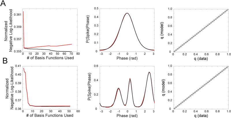
New method: Here we present a method to estimate probabilistic relationships between neural spiking activity and the phase of field oscillations using a generalized linear model (GLM) with an overcomplete basis of circular functions. We first use an L1-regularized maximum likelihood procedure to select an active set of regressors from the overcomplete set and perform model fitting using standard maximum likelihood estimation. An information theoretic model selection procedure is then used to identify an optimal subset of regressors and associated coefficients that minimize overfitting. To assess goodness of fit, we apply the time-rescaling theorem and compare model predictions to original data using quantile-quantile plots.

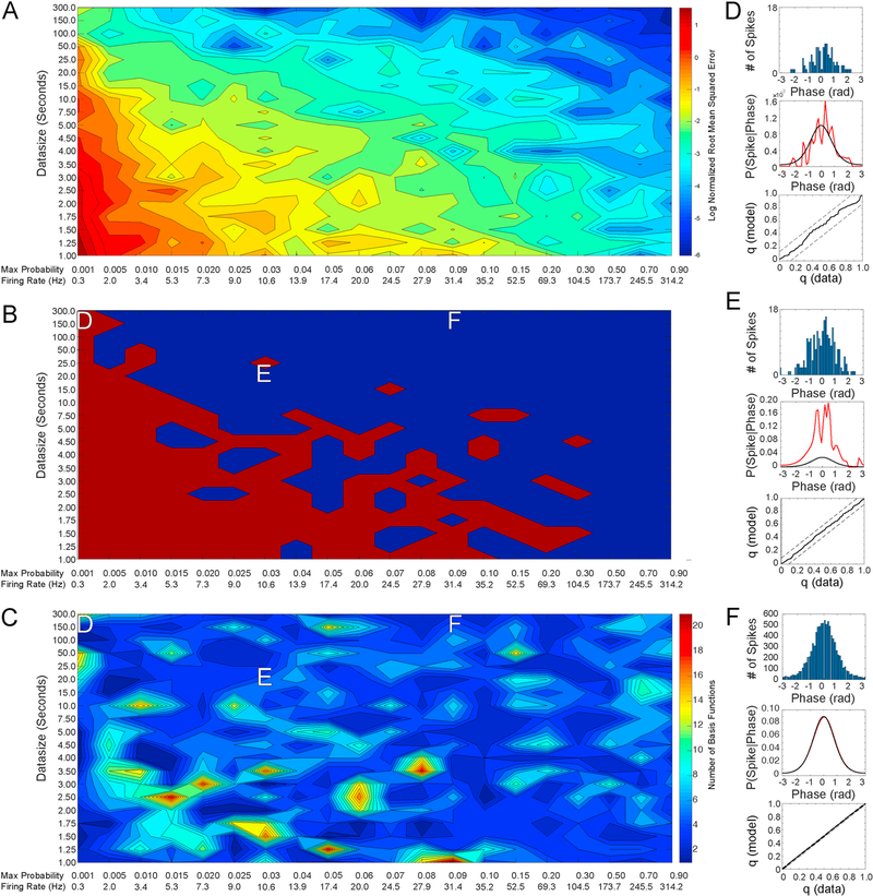
Results: Spike-phase relationships in synthetic data were robustly characterized. When applied to in vivo hippocampal data from an awake behaving rat, our method captured a multimodal relationship between the spiking activity of a CA1 interneuron, a theta (5-10 Hz) rhythm, and a nested high gamma (65-135 Hz) rhythm.

Comparison with existing methods: Previous methods for characterizing spike-phase relationships are often only suitable for unimodal relationships, impose specific relationship shapes, or have limited ability to assess the accuracy or fit of their characterizations.

Conclusions: This method advances the way spike-phase relationships are visualized and quantified, and captures multimodal spike-phase relationships, including relationships with multiple nested rhythms. Overall, our method is a powerful tool for revealing a wide range of neural circuit interactions.

Keywords: CA1; Gamma rhythm; Generalized linear model; Hippocampus; Interneuron; L1-regularization; Local field potential; Neural oscillations; Overcomplete basis; Point process modeling; Sparsity; Spike-phase relationship; Theta rhythm.

Fig. 1.

Illustration of select methods for visualizing and quantifying spike-phase relationships. A multimodal spike-phase relationship simulated from a mixture of Von Mises functions is shown in black. The estimated conditional probability of observing a spike given the phase of an oscillation using a single line function (blue), a single Von Mises function (green), a single sine function (purple), and 7 Von Mises functions assembled with our proposed workflow (red) is shown. In addition, we calculate the mean resultant length vector for the data, and show the estimated strength and preferred phase using this method (orange arrow). Our method is the only method capable of capturing the multimodal nature of this example spike-phase relationship. (For interpretation of the references to color in this figure legend, the reader is referred to the web version of this article.)

Fig. 2.

Illustration describing the methodological pipeline for predicting the probability of a spike given the phase of an oscillation. (A) Raw local field potential signal (gray), filtered signal in the theta (5–10 Hz) frequency range (red), and instantaneous phase of the theta oscillation (green) with corresponding spike times above (black tick marks). (B) A sample set of Von Mises basis functions used to construct model regressors. (C) Equation for calculating basis function weights using a ℓ₁-regularized generalized linear model, where the regularizer coefficient (λ_q) is systematically varied in order to selectively order the number of basis functions used. (D) Sample ordering of Von Mises basis functions used to characterize the data in Fig. 1, showing the active set of Von Mises functions with increasing model order complexity (gray). Our method selected seven functions as the optimal number of functions to represent the data (bottom), and we show the weighted combination of these functions for comparison (see also red line in Fig. 1). (E) Equation for calculating the weights for each basis function based upon the ordering determined in step C. (F) Normalized negative log likelihood (black) and penalized normalized negative log likelihood (red). (G) Sample Q-Q plot of actual and theoretical spiking data with associated 95% confidence interval. (H) Conditional probability estimated by the model that best characterizes the data while minimizing overfitting according to F. (For interpretation of the references to color in this figure legend, the reader is referred to the web version of this article.)

Fig. 3.

Model results for simulated unimodal (A) and multimodal (B) spike-phase relationships. Left: Normalized negative log likelihood (black) and penalized normalized negative log likelihood (red). Middle: Ground truth conditional probability function (black) and predicted conditional probability function (red). Right: Q-Q plots (solid line) with associated 95% confidence intervals (dashed lines). (For interpretation of the references to color in this figure legend, the reader is referred to the web version of this article.)

Fig. 4.

Model results given data sets with a range of different spiking probabilities and data sizes. (A) Log of the normalized root mean squared error (NRMSE) between conditional probability functions estimated by our method and the ground truth function used to generate the spiking data (see Eq. (20)). Maximum spiking probabilities (x-axis) range from 0.001 to 0.9 and data sizes (y-axis) range from 1 to 300 s (for method, see Section 2.9). Approximate firing rates, indicated below spike probabilities on the x-axis, are calculated from the total number of spikes in a 300 s interval. (B) Color map indicating whether ground truth spike-phase distributions and model predicted distributions are significantly different (red), assessed using a Kolmogorov–Smirnov test with a significance threshold of p=0.05. (C) The number of basis functions utilized after implementing model selection procedures. White labels D, E, and F within figures A–C indicate the spike probabilities and data sizes for examples in D–F. (D–F) Top: Distribution of simulated spikes across the phases of a 20 Hz oscillation. Middle: Ground truth conditional probability function (black) and predicted conditional probability function (red). Bottom: Q-Q plots (solid line) with associated 95% confidence intervals (dashed lines). (For interpretation of the references to color in this figure legend, the reader is referred to the web version of this article.)

Fig. 5.

Model results for spike-phase relationships to sinusoidal and non-sinusoidal signals. (A) Single cycle of a simulated sinusoidal and non-sinusoidal signal. Distribution of phases for 60 s of a (B) sinusoidal (blue) and (C) non-sinusoidal (red) 8 Hz signal. While the sinusoidal signal contains a uniform distribution of phases, the non-sinusoidal condition contains a larger number of phases centered around 0 radians. (D–F) The estimated probability of observing a spike given the phase of a sinusoidal (dashed cyan) and non-sinusoidal (dashed magenta) oscillation for three different conditions: (D) a unimodal spike-phase relationship centered at 0 radians where there is a higher sampling of phases in our non-sinusoidal signal, (E) a unimodal spike-phase relationship centered at π radians where there is a lower sampling of phases in our non-sinusoidal signal, and (F) a condition in which there is an equal probability (0.035) of observing a spike at every phase that is based upon the average firing rate in D and E. Ground truth conditional probability functions for D–F are shown in black dashed lines. Corresponding Q-Q plots (colored dashed lines) with associated 95% confidence intervals (black dashed lines) are shown directly below (D–F). (For interpretation of the references to color in this figure legend, the reader is referred to the web version of this article.)

Fig. 6.

Rat hippocampal neuron data. (A) Histogram of interneuron spikes across the phases of a 5–10 Hz theta oscillation (black, left axis) and a histogram presenting the distribution of theta phases from the filtered LFP (blue, right axis). (B) Representative segment of raw local field potential data (gray), theta phase (green), and spiking times (black tick marks). (C) Raw local field potential data (gray), 5–10 Hz theta filtered local field potential (red), gamma filtered local field potential (blue), and spike times (black tick marks). (D) Normalized negative log likelihood (black) and AIC penalized normalized negative log likelihood (red). (E) Estimated conditional probability of observing a spike given the phase of theta using one basis function (red) and twenty-two basis functions (black). (F) Raw local field potential data (gray), theta filtered local field potential (red), single basis function theta conditional intensity function (magenta), and spike times (black tick marks). (G and H) Q-Q plots of actual and theoretical spiking data for (G) 300 s and (H) isolated 10 s intervals using the model selected by the workflow. (I) Raw local field potential data (gray), gamma filtered local field potential (blue), gamma conditional intensity function (cyan) and spike times (black tick marks). (For interpretation of the references to color in this figure legend, the reader is referred to the web version of this article.)

References

1. Akaike H, 1974. A new look at the statistical model identification. IEEE Trans. Autom. Control 19 (6), 716–723.
1. Aoi MC, Lepage KQ, Kramer MA, Eden UT, 2015. Rate-adjusted spike—LFP coherence comparisons from spike-train statistics. J. Neurosci. Methods 240, 141–153. - PMC - PubMed
1. Barbieri R, Frank LM, Quirk MC, Solo V, Wilson MA, Brown EN, 2002. Construction and analysis of non-Gaussian spatial models of neural spiking activity. Neurocomputing 44, 309–314.
1. Barbieri R, Quirk MC, Frank LM, Wilson MA, Brown EN, 2001. Construction and analysis of non-Poisson stimulus-response models of neural spiking activity. J. Neurosci. Methods 105 (1), 25–37. - PubMed
1. Belloni A, Chernozhukov V, et al., 2013. Least squares after model selection in high-dimensional sparse models. Bernoulli 19 (2), 521–547.
Publication types