Estimates of the Heritability of Human Longevity Are Substantially Inflated due to Assortative Mating

Abstract

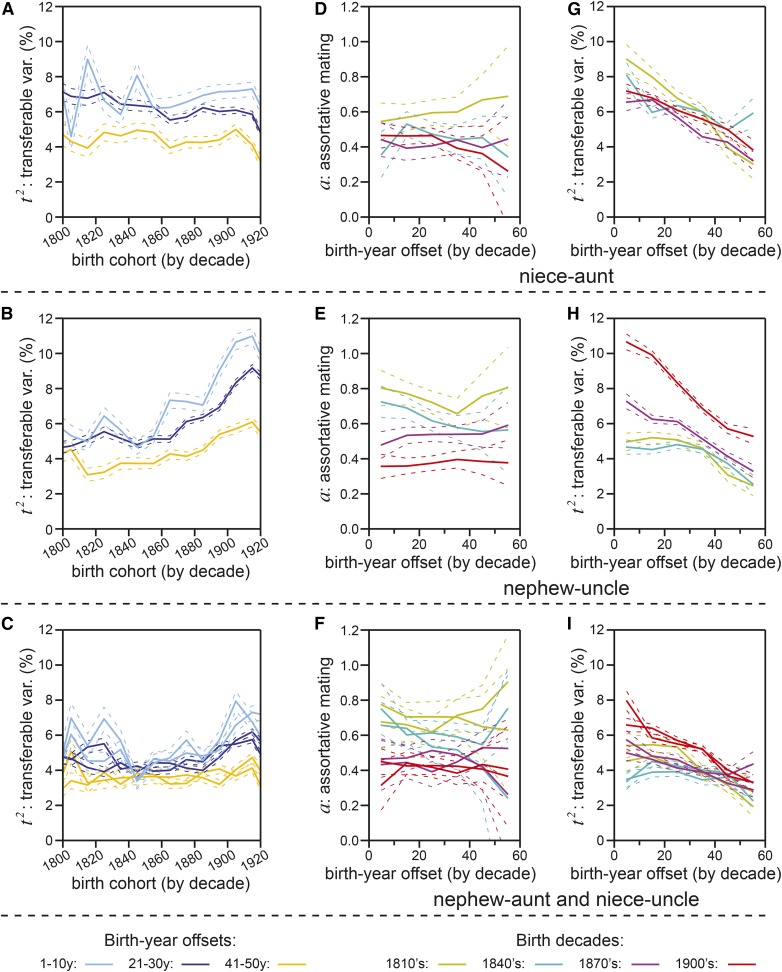
Human life span is a phenotype that integrates many aspects of health and environment into a single ultimate quantity: the elapsed time between birth and death. Though it is widely believed that long life runs in families for genetic reasons, estimates of life span "heritability" are consistently low (∼15-30%). Here, we used pedigree data from Ancestry public trees, including hundreds of millions of historical persons, to estimate the heritability of human longevity. Although "nominal heritability" estimates based on correlations among genetic relatives agreed with prior literature, the majority of that correlation was also captured by correlations among nongenetic (in-law) relatives, suggestive of highly assortative mating around life span-influencing factors (genetic and/or environmental). We used structural equation modeling to account for assortative mating, and concluded that the true heritability of human longevity for birth cohorts across the 1800s and early 1900s was well below 10%, and that it has been generally overestimated due to the effect of assortative mating.

Keywords: assortative mating; heritability; human; life span.

Figure 1

Properties of the Ancestry data set. (A) An overview of the SAP, showing the fraction of the data meeting the most basic requirements for this analysis (pedigree membership and assignment to a birth cohort: left) and the composition of the SAP in terms of subtrees (almost the entire pedigree-linked population being members of a single tree: right). (B) The number of individuals born per decade. Limited to nonsingleton individuals with known year-of-birth. (C) The number of individuals born per year. All nonsingleton individuals with known year-of-birth (yellow), and individuals who additionally have year-of-death data and have tree connections to both parents, to a child, and to a spouse (purple). The panels on the left depict birth years 1700–1749; the panels on the right depict birth years 1850–1899. (D) Enrichment for “rounded” years-of-birth: for each decade, the log₂ of the ratio between mean number of births for years ending in “0” or “5,” and the mean number of births for other years is plotted on the y-axis. Colors as in (C). (E) Male-to-female gender ratio for nonsingleton individuals with known year-of-birth, plotted by decade-of-birth. (F) Percentages of the nonsingleton, known-year-of-birth population with spouses (yellow), with at least one child (purple), and with both parents (cyan), per birth-decade. (G) Percentages of the nonsingleton, known-year-of-birth population with known year-of-death (blue), or additionally with tree connections to both parents, to a child, and to a spouse (purple), per birth-decade. (H) Percentages of the nonsingleton, known-year-of-birth population with geographical data at any resolution for birth (red), for death (also requiring a known year-of-death; purple), and for both birth and death (yellow). (I) Percentages of the nonsingleton, known-year-and-geography-of-birth population born in the contiguous U.S.A. (red), Europe (blue), or elsewhere (cyan), per birth-decade. pct. of pop., percent of population; SAP, set of aggregated and anonymized pedigrees.

Figure 2

A summary of our structural equation model. (A) A traditionally drawn pedigree of a nuclear family, with two parents (father: F and mother: M) and two children (sister: S and brother: B). As per convention, squares represent males and circles represent females. (B) The pathway diagram for our structural equation model’s description of the phenotypic correlation between the two siblings from the family depicted in (A). Please note the different convention for node shapes in pathway diagrams for structural equation models: here, squares represent observable states (phenotypes), while circles represent latent states. See Supplemental Text, section 1 for more discussion of these diagrams and a full explanation of the model.

Figure 3

Life span correlations with in-law relatives and patterns of remote relative correlations reveal substantial assortative mating for factors affecting longevity. (A) Life span correlations for siblings (y-axis); x-axis: the birth-decade of the proband. The sibling of each proband was required to be born 1–10 years prior to that proband. Gender-specific correlations between male–male (MM; cyan), female–female (FF; red), female–male (FM; magenta), and male–female (MF; yellow) sibling-pairs were calculated separately. Dotted lines indicate estimate SE. The nominally estimated heritability values are shown on the right-hand y-axis. (B) Life span correlations for first cousins, calculated and plotted as in (A). (C) Life span correlations for female–male sibling-pairs [FM; magenta; reproduced from (A)] and spouse-pairs (orange), calculated and plotted as in (A). (D) Life span correlations for siblings-in-law, calculated and plotted as in (A). (E) Life span correlations for first-cousins-in-law, calculated and plotted as in (A). (F) A theoretical plot illustrating the linearity between additive relatedness (x-axis) vs. phenotypic correlation (y-axis) that is assumed across relative types by the nominal heritability model (see Supplemental Text, section 2). Dots indicate particular relationship types; the dashed gray line indicates the continuous function. (G) A theoretical plot illustrating the amplifying effects of assortative mating (a) on phenotypic correlations. Axes as in (F). For various values of a, dots indicate particular relationship types [colored as in (F)]; dashed gray lines indicate the continuous functions (see Supplemental Text, section 2). (H) The observed relationships between additive relatedness (x-axis) and life span correlations (y-axis) for four remote relative types, all relatives born 1–10 years prior to the proband. Dots indicate the mean value for decade birth cohorts, 1800–1920. Vertical lines indicate the SD of correlation values across those decades. Each panel displays estimates for a particular gender pair, colored as in (A). Dashed gray lines indicated a nominal (linear) extrapolation through piblings. Siblings are omitted from this plot due to the confounding effects of shared-household environment (see Supplemental Text, sections 1.4 and 2.2).

Figure 4

Structural equation modeling of sibling-in-law networks reveals a substantial role for assortative mating and a diminished role for transferable variance (t²) in human life span. (A) Life span correlations for cosiblings-in-law of the sib-law-sib variety (see Results), calculated and plotted as in Figure 3A. (B) Life span correlations for cosiblings-in-law of the law-sib-law variety (the sibling of a sibling’s spouse, see Results), calculated and plotted as in Figure 3A. (C) Life span correlations for siblings-in-law (reproduced from Figure 3D; shown for direct comparison to (A and B). (D) Pathway diagrams for the application of our structural equation model to the three relative types in (A–C) (see Supplemental Text, section 1 for details). (E). Transferable variance (t²), calculated from the data in (A–C) (see Supplemental Text, section 3.3 for solving method). Colored as in Figure 3A. (F) The assortative mating coefficient (a), calculated from the data in (A–C) (see Supplemental Text, section 3.4 equation 43 for solving method). Colored as in Figure 3A. (G) The inheritance coefficient (β), calculated from the data in (A–C) (see Supplemental Text, section 3.5 for solving method). Colored as in Figure 5A. (H) The correlative effect of nontransferable shared childhood environment (shared-env. corr.) on sibling life spans (c_sib; y-axis), along with the relevant pathway diagram. See Supplemental Text, section 3.6 for solving method. Colored as in Figure 3A. (I) The correlative effect of nontransferable shared adult environment on spouses’ life spans (c_sp; y-axis), along with the relevant pathway diagram. See Supplemental Text, section 3.6 for solving method. Female–male (FM; magenta) and male–female (MF; yellow) spouse-pairs are plotted, with the first-listed gender of each pair being the proband (younger individual).

Figure 5

Correlations between remote in-law relatives confirm a substantial role for assortative mating and a diminished role for transferable variance (t²) in human life span. (A) The assortative mating coefficient (a), calculated via division of pibling-in-law life span correlation by pibling life span correlation (see Supplemental Text, section 3.4 equation 44 for solving method). (B) The assortative mating coefficient (a), calculated via division of first-cousin-in-law life span correlation by first cousin life span correlation. (C) The assortative mating coefficient (a), calculated via division of first-cousin-once-removed-in-law life span correlation by first-cousin-once-removed life span correlation. (D) Transferable variance (var.) (t²), calculated by the assortment-correction method (see Supplemental Text, section 3.7 for solving method) using pibling correlations and a estimates from (A). (E) Transferable variance (t²), calculated by the assortment-correction method using first-cousin correlations and a estimates from (B). (F) Transferable variance (t²), calculated by the assortment-correction method using first-cousin-once-removed correlations and a estimates from (C). (A–F) Colored as in Figure 3A.

Figure 6

Assortment-corrected estimates of transferable variance (var.) (t²) diminish as relatives’ birth cohorts diverge. (A) Niece–aunt transferable variance (t²) (solid lines) calculated by the assortment-correction method (see Supplemental Text, section 3.7 for solving method) for each decade-long niece birth cohort, for aunts whose birth years were offset from their nieces by 1–10 years (cyan), 21–30 years (blue), or 41–50 years (yellow). SE of estimates are shown as dotted lines. (B) Nephew–uncle transferable variance (t²), calculated and plotted as in (A). (C) Nephew–aunt and niece–uncle transferable variances (t²), each calculated and plotted together as in (A). (D) The assortative mating coefficient (a; y-axis), calculated via division of niece–aunt-in-law life span correlation by niece–aunt life span correlation (see Supplemental Text, section 3.4 equation 44 for solving method), plotted for niece–aunt pairs of varying birth-year offsets (x-axis indicates the number of years prior to the niece’s birth the aunt was born) for four decade-long niece birth cohorts: 1810s (yellow), 1840s (cyan), 1870s (magenta), and 1900s (red). Dotted lines show SE. (E) The assortative mating coefficient (a) vs. birth-year offsets for nephew–uncle and nephew–uncle-in-law pairs, calculated and plotted as in (D). (F) The assortative mating coefficient (a) vs. birth-year offsets for niece–uncle and niece–uncle-in-law pairs, or nephew–aunt and nephew–aunt-in-law pairs, calculated for each and plotted together as in (D). (G) Niece–aunt transferable variance (t²) calculated as in (A), plotted by birth-year offset as in (D). (H) Nephew–uncle transferable variance (t²) calculated as in (B), plotted by birth-year offset as in (E). (I) Niece–uncle and nephew–aunt transferable variances (t²) calculated as in (C), plotted by birth-year offset as in (F).

References

1. Ancestry.com and Board for Certification of Genealogists , 2014. Genealogy Standards. Ancestry.com, Provo, UT.
1. Becker G., Tomes N., 1986. Human capital and the rise and fall of families. J. Labor Econ. 4: S1–S39. 10.1086/298118 - DOI - PubMed
1. Björklund A., Eriksson T., Jäntti M., Raaum O., Österbacka E., 2002. Brother correlations in earnings in Denmark, Finland, Norway and Sweden compared to the United States. J. Popul. Econ. 15: 757–772. 10.1007/s001480100095 - DOI
1. Braveman P. A., Cubbin C., Egerter S., Chideya S., Marchi K. S., et al. , 2005. Socioeconomic status in health research: one size does not fit all. JAMA 294: 2879–2888. 10.1001/jama.294.22.2879 - DOI - PubMed
1. Brooks-Wilson A. R., 2013. Genetics of healthy aging and longevity. Hum. Genet. 132: 1323–1338. 10.1007/s00439-013-1342-z - DOI - PMC - PubMed
Publication types