A Comprehensive Review of Optical Stretcher for Cell Mechanical Characterization at Single-Cell Level

Abstract

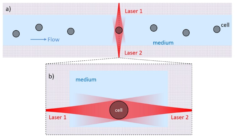
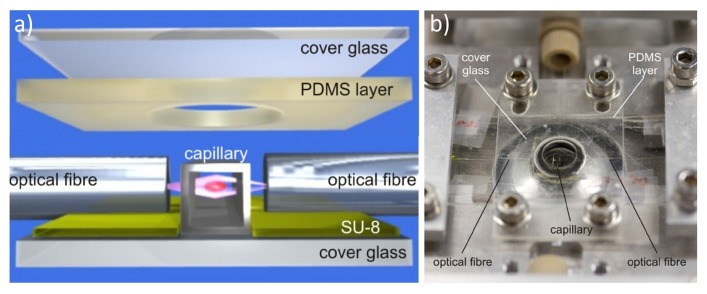
This paper presents a comprehensive review of the development of the optical stretcher, a powerful optofluidic device for single cell mechanical study by using optical force induced cell stretching. The different techniques and the different materials for the fabrication of the optical stretcher are first summarized. A short description of the optical-stretching mechanism is then given, highlighting the optical force calculation and the cell optical deformability characterization. Subsequently, the implementations of the optical stretcher in various cell-mechanics studies are shown on different types of cells. Afterwards, two new advancements on optical stretcher applications are also introduced: the active cell sorting based on cell mechanical characterization and the temperature effect on cell stretching measurement from laser-induced heating. Two examples of new functionalities developed with the optical stretcher are also included. Finally, the current major limitation and the future development possibilities are discussed.

Keywords: mechanical properties characterization; microfluidics; optical stretcher; optofluidics; single-cell analysis.

Figure 1

Schematic structure of an optical stretcher. (a) Top view of the central fluidic channel with flowing cells and a single cell trapped in the middle of the two opposing laser beams; (b) Cross section of the trapping area as indicated by the dash line in (a). The two opposite laser beams are positioned close to the channel floor.

Figure 2

The structure of the discrete-element optical stretcher. (a) 3D rendering of the constituent components and their positions; (b) The finished system is mounted on a microscope plate. Figure reproduced from Reference [29] with permission from Optical Society of America.

Figure 3

The chip geometry of the double glass layer assembled optical stretcher. The two glass layer are etched asymmetrically, the top one for large part of the fiber and the entire fluidic channel, the bottom one with shallow grooves for fiber alignment. The misalignment between these two layers show the robustness of this new etching layout. Figure reproduced from Reference [25] under CC-BY 3.0 license.

Figure 4

The polymeric assembled optical stretcher. (a) SEM image of the Ni shim at the area where the fiber grooves meet the channel. Higher position of the fiber grooves with respect to the central channel will lead to the lower position of the fibers after insertion; (b) Bright filed microscope image of the chip at the same area with a photonic crystal fiber (left) and single mode fiber (right) inserted; (c) The finished chip ready for use. The three inlets are for hydrodynamic focusing purpose. Figure reproduced from Reference [30] under CC-BY 4.0 license.

Figure 5

(a) Schematic representation of the three-layer technology for the monolithic optical stretcher fabrication. The central fused silica glass is machined by Femtosecond Laser Irradiation followed by Chemical Etching (FLICE) technique for the central channel and then sealed on both sides with two polished glass slides; (b) Microscope image of the straight microfluidic channel with pairs of waveguides beside it; (c) The finished chip is pigtailed with optical fibers and connected with external tubing through Luer connectors. Figure reproduced from Reference [29] with permission from Optical Society of America.

Figure 6

Scheme of the optical field determination from a Gaussian laser beam with the paraxial ray optics approach. (a) The power carried by each ray, is calculated as the integral of the beam intensity, as a function of the radial coordinate within the area of the annulus associated to the ray; (b) The amplitude A(ρ, z) and the (c) curvature radius R(ρ, z) along the axis z are calculated, which will be exploited respectively for the evaluation of the power and the propagation direction of each ray.

Figure 7

Coordinate system for a single ray interacting with a particle. (a) A single rays from a Gaussian laser beams hits on the surface of a particle. The locations of the laser beam and particle can be random. The incident plane is defined by the ray and the normal direction of the particle at the hitting point and is indicated by the gray area; (b) the single ray undergoes multiple reflections and refractions on the boundary of the particle.

Figure 8

Polar plots of the calculated optical stress distribution on the surface of the particle. The Gaussian laser beam has beam waist of 3.1 µm and wavelength of 1.07 µm and carries optical power of 10 mW. The refractive index of the particle is 1.37 and medium 1.33. The distance between the particle center and the beam waist (either one laser or two lasers) is indicated in each panel together with the diameter of the particle. (a–c) show the optical stress from left side laser radiation, right side laser radiation and both side laser radiation respectively; From (d) to (i), the two-side laser irradiation is considered; (d–f) show the optical stress distribution change with particle size increase; (g–i) show the optical stress distribution change with distance increase.

Figure 9

Flow chart of continuous cell stretching procedure.

Figure 10

Illustration of the image analysis steps. (a) Phase contrast microscope image of a single cell. The center point (red color) of the cell is manually selected and the circular border (light blue color) for the polar transformation is determined by the original rectangular image border; (b) The polar-transformed image; (c) shows a plot of the gray-scale intensity along the green vertical line appearing in (b). The raw data (red line) is smoothed by Fourier filtering (blue line); (d) shows the first derivative of the blue-line (intensity) and the red circle shows the point identified as minimum, identified as belonging to cell border; (e) by repeating the same procedure for all the polar angles, the cell border is reconstructed on the polar image and (f) then transformed back to original image.

Figure 11

Single cell optical stretching. (a) Cell dimension variation during optical stretching together with the laser power profile (b): P${}_T$ is trapping laser power of 25 mW per side and P${}_S$ is stretching power of 1.5 W per side. X-axis is along the laser beam and Y-axis along the cell flowing direction; (c,d) show the phase contrast microscope images of the same cell trapped and stretched respectively. Green contours are cell borders identified by the recognition algorithm. Scale bars in both (b,c) are 10 µm. The cell sample is human breast cancer cell MCF7.

Figure 12

Optical stretching of single red blood cell (RBC). (a) Microscope images of RBCs stretched at increasing optical powers; (b) Optical deformation of RBCs in terms of elongation along laser axis and contraction in the perpendicular direction at different stretching power. The laser power is the total power for both laser beams. Experimental data is fitted with theoretical prediction from the linear elastic membrane theory. Figure reproduced from Reference [45] with permission from Optical Society of America.

Figure 13

Optical stretching of vesicles. Microscope image of a vesicle trapped at low power (a) and deformed at high power (b); (c) The major axis strain of vesicles under 4 s stretching at various total powers. Figure reproduced from Reference [62] with permission from Royal Society of Chemistry.

Figure 14

Optical stretching of a single MCF7 cell. The laser power is for each side and the cell contour is recognized by the edge detection algorithm in Figure 10.

Figure 15

Optical deformability of normal, cancerous, and metastatic breast epithelial cells. (a) The three populations of the MCF cell and (b) the two populations of the MDA-MB-231 cell are clearly distinguishable. Curves represent the fitting of normal distribution. Figure reproduced with permission from Reference [23] with permission from Prof. Guck.

Figure 16

Active cell sorting chip design. (a) Microscope image of the internal structure of the cell sorting microchip. Scale bar: 100 µm; (b) The finished chip with fibers pigtailed and tubing connected is very compact. Scale bar: 1 cm; (c) Schematic of the experimental setup. Figure reproduced from Reference [24] with permission from Royal Society of Chemistry.

Figure 17

Laser writing geometry optimization for internal channel surface roughness control. Figure reproduced from Reference [24] with permission from Royal Society of Chemistry.

Figure 18

Cell sorting efficiency check. Characterization of the cellular size (a) and optical deformability (b) of two cell lines, A375MC2 and A375P; (c) Normalized cellular distributions as a function of their optical deformations from experiment data in (b). The whole area under each cell curve is set equal representing the same concentration. By defining a deformation threshold, a sub-population of A375MC2 can be enriched by collecting cells with higher deformability; (d) The ratio of A375MC2 in the collected cell sample and the ratio of cells in the initial sample that are expected to exhibit deformability higher than the threshold (acceptance rate) versus the defined threshold value. Figure reproduced from Reference [24] with permission from Royal Society of Chemistry.

Figure 19

Spatial temperature profile in an optical stretcher. (a) Color image of the temperature increase from the two opposing laser beams in the optical stretcher. The imaging plane is the channel cross section through the center of the trap and the power of each laser beam is 1 W; (b) Line scan of the temperature along the dashed line in (a). Figure reproduced from Reference [71] with permission from Optical Society of America.

Figure 20

Temporal revolution of the temperature from the laser radiation in the optical stretcher. The laser is turned on at t = 2 s and has a total power of 2 W. Figure reproduced from Reference [71] with permission from Optical Society of America.

Figure 21

Heat shock impact on cell viability with different laser power (temperature) and time duration. The figure was realized exploiting the data reported in Reference [72].

Figure 22

Active temperature control for optical stretcher. (a) Two additional fibers are added and positioned near the two opposing stretching fibers for temperature control; (b) Another laser is coupled into one of the two stretching fibers for temperature control. Figure reproduced from Reference [76,79] under CC-BY 3.0 license.

Figure 23

Temperature effect on cell optical deformation. Temperature is changed during the stretching measurement by using the two additional heating fibers (P${}_{heat}$), see Figure 22a, while keeping the stretcher power (P${}_{stretch}$) constant. Figure reproduced from Reference [76] under CC-BY 3.0 license.

Figure 24

Acoustic prefocusing for optical stretcher. (a) Schematic illustration of the all glass microchip with both acoustic actuation (the black dash lines) driven by the underneath piezo ceramic and optical radiation (the red shaded area) emanating from the integrated waveguides. The microfluidic channel has a square cross section, 150 µm × 150 µm; (b) Microscope image of polystyrene beads trapped by acoustic wave in the middle of the microfluidic channel both horizontally and vertically (all beads are in the same focus); (c) Microscope image of red blood cells prefocused with acoustic wave for continuous optical stretching. Two opposing lasers from the waveguides are visible because of the light scattering.

Figure 25

Optical cell rotator. (a) Illustration of the cell rotator realized in the two opposing laser radiation with an optical stretcher; (b) Microscope image sequences showing precise control of the cell orientation with red blood cell and HL60 cell. Figure reproduced from Reference [83] under CC-BY 4.0 license.

References

1. Suresh S. Biomechanics and biophysics of cancer cells. Acta Mater. 2007;55:3989–4014. doi: 10.1016/j.actamat.2007.04.022. - DOI - PMC - PubMed
1. Bao G., Suresh S. Cell and molecular mechanics of biological materials. Nat. Mater. 2003;2:715–725. doi: 10.1038/nmat1001. - DOI - PubMed
1. Fletcher D.A., Mullins R.D. Cell mechanics and the cytoskeleton. Nature. 2010;463:485–492. doi: 10.1038/nature08908. - DOI - PMC - PubMed
1. Moeendarbary E., Harris A.R. Cell mechanics: Principles, practices, and prospects. Wiley Interdiscip. Rev. Syst. Biol. Med. 2014;6:371–388. doi: 10.1002/wsbm.1275. - DOI - PMC - PubMed
1. Kumar S., Weaver V. Mechanics, malignancy, and metastasis: The force journey of a tumor cell. Cancer Metastas. Rev. 2009;28:113–127. doi: 10.1007/s10555-008-9173-4. - DOI - PMC - PubMed
LinkOut - more resources