

Segmentation of the Proximal Femur from MR Images using Deep Convolutional Neural Networks
- PMID: 30405145
- PMCID: PMC6220200
- DOI: 10.1038/s41598-018-34817-6
Segmentation of the Proximal Femur from MR Images using Deep Convolutional Neural Networks
Abstract
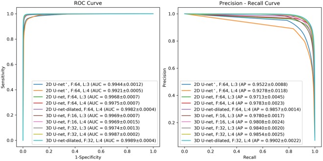
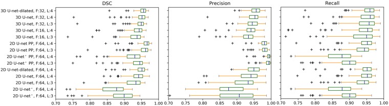
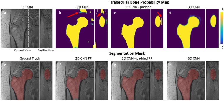
Magnetic resonance imaging (MRI) has been proposed as a complimentary method to measure bone quality and assess fracture risk. However, manual segmentation of MR images of bone is time-consuming, limiting the use of MRI measurements in the clinical practice. The purpose of this paper is to present an automatic proximal femur segmentation method that is based on deep convolutional neural networks (CNNs). This study had institutional review board approval and written informed consent was obtained from all subjects. A dataset of volumetric structural MR images of the proximal femur from 86 subjects were manually-segmented by an expert. We performed experiments by training two different CNN architectures with multiple number of initial feature maps, layers and dilation rates, and tested their segmentation performance against the gold standard of manual segmentations using four-fold cross-validation. Automatic segmentation of the proximal femur using CNNs achieved a high dice similarity score of 0.95 ± 0.02 with precision = 0.95 ± 0.02, and recall = 0.95 ± 0.03. The high segmentation accuracy provided by CNNs has the potential to help bring the use of structural MRI measurements of bone quality into clinical practice for management of osteoporosis.
Conflict of interest statement
G.C. has a pending patent application (# 62/593,626) filed by the University of Iowa. G.C. shares the invention with Punam Saha. Specific aspects of this manuscript were not covered in the patent application. The other authors do not have conflict of interests to disclose.
Figures


Similar articles
-
Fully automatic, multiorgan segmentation in normal whole body magnetic resonance imaging (MRI), using classification forests (CFs), convolutional neural networks (CNNs), and a multi-atlas (MA) approach.Med Phys. 2017 Oct;44(10):5210-5220. doi: 10.1002/mp.12492. Epub 2017 Aug 31. Med Phys. 2017. PMID: 28756622
-
Semantic segmentation of the multiform proximal femur and femoral head bones with the deep convolutional neural networks in low quality MRI sections acquired in different MRI protocols.Comput Med Imaging Graph. 2020 Apr;81:101715. doi: 10.1016/j.compmedimag.2020.101715. Epub 2020 Mar 5. Comput Med Imaging Graph. 2020. PMID: 32240933
-
Using 2D U-Net convolutional neural networks for automatic acetabular and proximal femur segmentation of hip MRI images and morphological quantification: a preliminary study in DDH.Biomed Eng Online. 2024 Oct 5;23(1):98. doi: 10.1186/s12938-024-01291-3. Biomed Eng Online. 2024. PMID: 39369206 Free PMC article.
-
A deep learning-based approach to automatic proximal femur segmentation in quantitative CT images.Med Biol Eng Comput. 2022 May;60(5):1417-1429. doi: 10.1007/s11517-022-02529-9. Epub 2022 Mar 24. Med Biol Eng Comput. 2022. PMID: 35322343 Review.
-
Review of different convolutional neural networks used in segmentation of prostate during fusion biopsy.Cent European J Urol. 2025;78(1):23-39. doi: 10.5173/ceju.2024.0064. Epub 2025 Mar 21. Cent European J Urol. 2025. PMID: 40371421 Free PMC article. Review.
Cited by
-
Improving Quantitative Magnetic Resonance Imaging Using Deep Learning.Semin Musculoskelet Radiol. 2020 Aug;24(4):451-459. doi: 10.1055/s-0040-1709482. Epub 2020 Sep 29. Semin Musculoskelet Radiol. 2020. PMID: 32992372 Free PMC article. Review.
-
Classification of negative and positive 18F-florbetapir brain PET studies in subjective cognitive decline patients using a convolutional neural network.Eur J Nucl Med Mol Imaging. 2021 Mar;48(3):721-728. doi: 10.1007/s00259-020-05006-3. Epub 2020 Sep 2. Eur J Nucl Med Mol Imaging. 2021. PMID: 32875431 Free PMC article.
-
Deep Learning-Based Approach for Emotion Recognition Using Electroencephalography (EEG) Signals Using Bi-Directional Long Short-Term Memory (Bi-LSTM).Sensors (Basel). 2022 Apr 13;22(8):2976. doi: 10.3390/s22082976. Sensors (Basel). 2022. PMID: 35458962 Free PMC article.
-
Automatic prostate and prostate zones segmentation of magnetic resonance images using DenseNet-like U-net.Sci Rep. 2020 Aug 31;10(1):14315. doi: 10.1038/s41598-020-71080-0. Sci Rep. 2020. PMID: 32868836 Free PMC article.
-
Nonlinear voxel-based finite element model for strength assessment of healthy and metastatic proximal femurs.Bone Rep. 2020 Apr 1;12:100263. doi: 10.1016/j.bonr.2020.100263. eCollection 2020 Jun. Bone Rep. 2020. PMID: 32322609 Free PMC article.
References
-
- Genant Harry K., Engelke Klaus, Fuerst Thomas, Glüer Claus-C., Grampp Stephan, Harris Steven T., Jergas Michael, Lang Thomas, Lu Ying, Majumdar Sharmila, Mathur Ashwini, Takada Masa. Noninvasive assessment of bone mineral and structure: State of the art. Journal of Bone and Mineral Research. 2009;11(6):707–730. doi: 10.1002/jbmr.5650110602. - DOI - PubMed
-
- Okazaki Narihiro, Chiba Ko, Taguchi Kenji, Nango Nobuhito, Kubota Shogo, Ito Masako, Osaki Makoto. Trabecular microfractures in the femoral head with osteoporosis: Analysis of microcallus formations by synchrotron radiation micro CT. Bone. 2014;64:82–87. doi: 10.1016/j.bone.2014.03.039. - DOI - PubMed
Publication types
MeSH terms
Grants and funding
LinkOut - more resources
Full Text Sources
Other Literature Sources
Medical
