Harnessing olfactory bulb oscillations to perform fully brain-based sleep-scoring and real-time monitoring of anaesthesia depth

Abstract

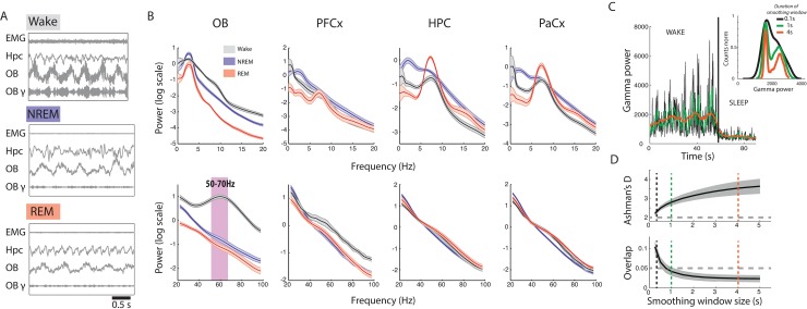
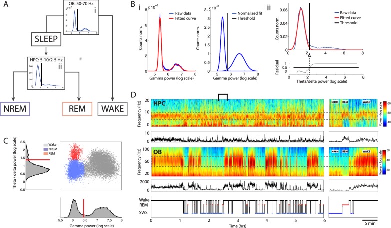
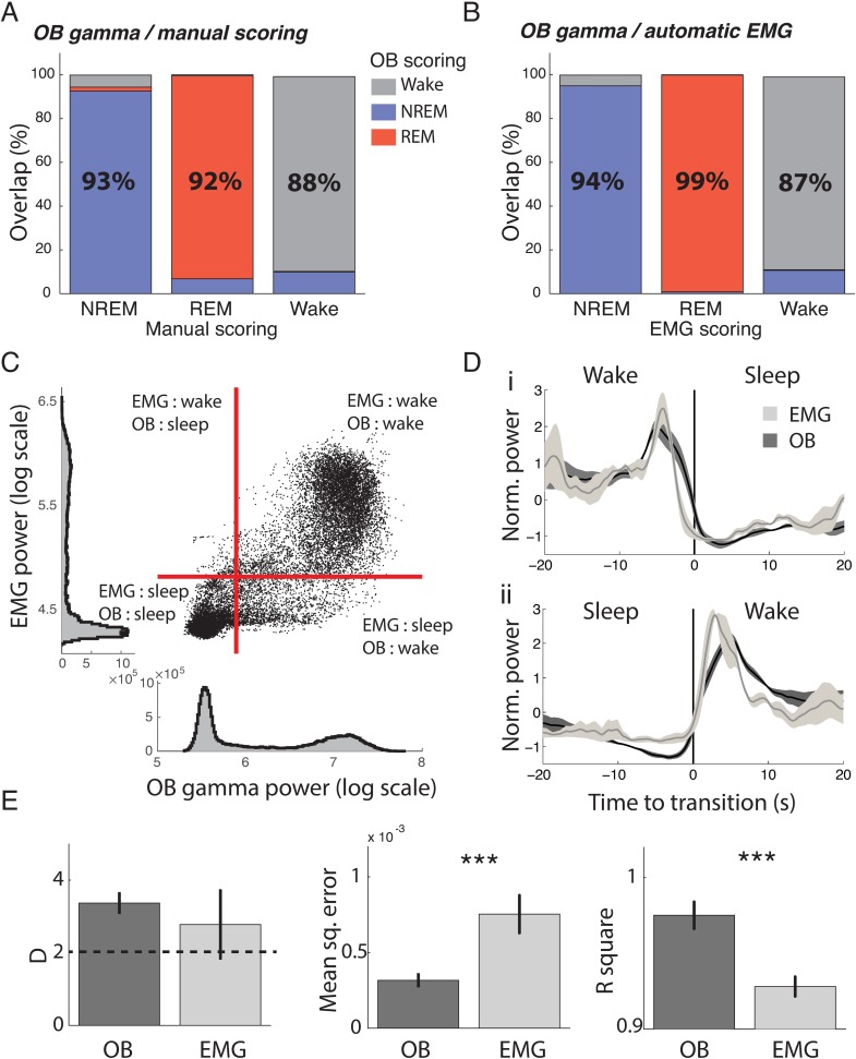
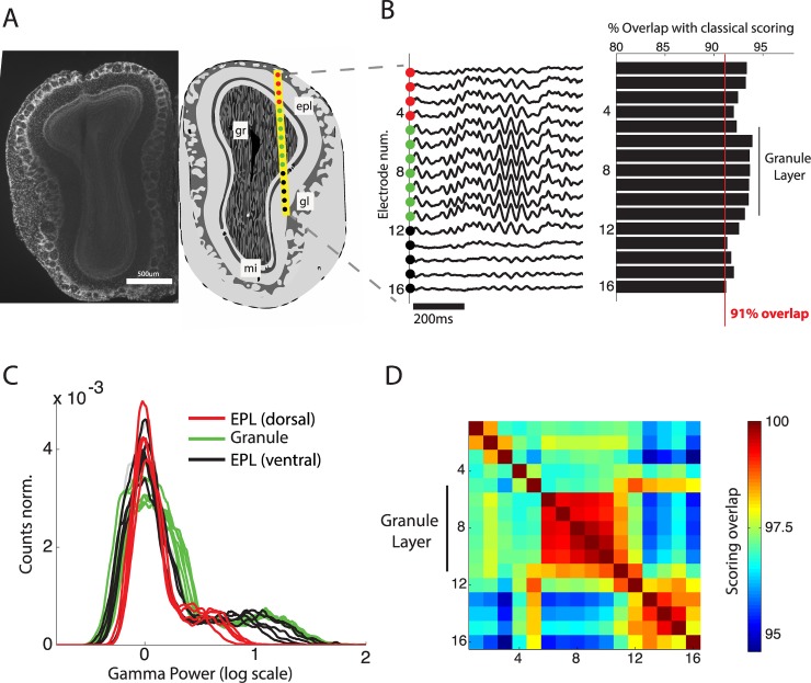
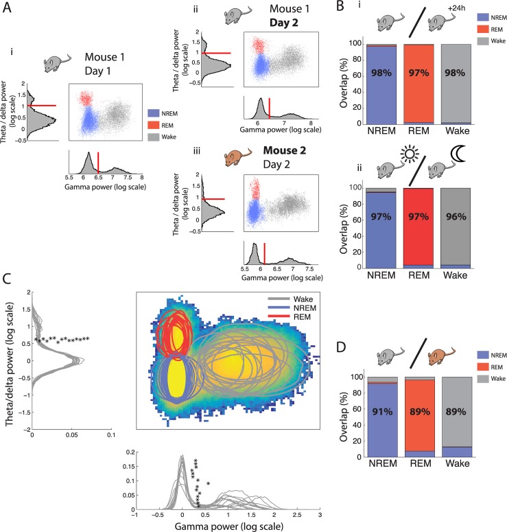
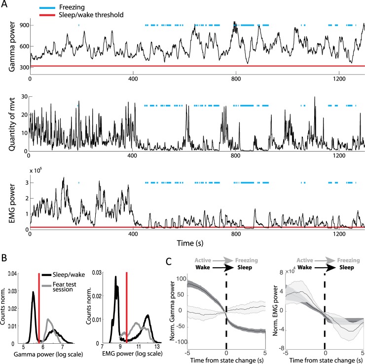
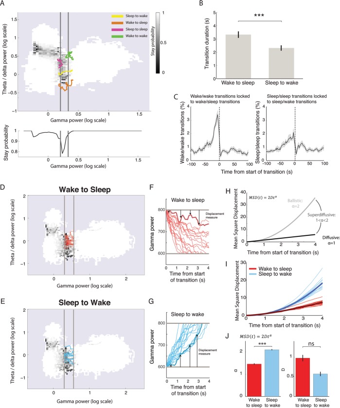
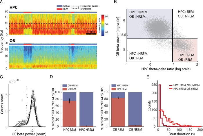
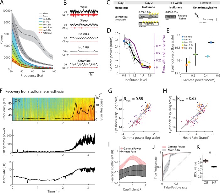
Real-time tracking of vigilance states related to both sleep or anaesthesia has been a goal for over a century. However, sleep scoring cannot currently be performed with brain signals alone, despite the deep neuromodulatory transformations that accompany sleep state changes. Therefore, at heart, the operational distinction between sleep and wake is that of immobility and movement, despite numerous situations in which this one-to-one mapping fails. Here we demonstrate, using local field potential (LFP) recordings in freely moving mice, that gamma (50-70 Hz) power in the olfactory bulb (OB) allows for clear classification of sleep and wake, thus providing a brain-based criterion to distinguish these two vigilance states without relying on motor activity. Coupled with hippocampal theta activity, it allows the elaboration of a sleep scoring algorithm that relies on brain activity alone. This method reaches over 90% homology with classical methods based on muscular activity (electromyography [EMG]) and video tracking. Moreover, contrary to EMG, OB gamma power allows correct discrimination between sleep and immobility in ambiguous situations such as fear-related freezing. We use the instantaneous power of hippocampal theta oscillation and OB gamma oscillation to construct a 2D phase space that is highly robust throughout time, across individual mice and mouse strains, and under classical drug treatment. Dynamic analysis of trajectories within this space yields a novel characterisation of sleep/wake transitions: whereas waking up is a fast and direct transition that can be modelled by a ballistic trajectory, falling asleep is best described as a stochastic and gradual state change. Finally, we demonstrate that OB oscillations also allow us to track other vigilance states. Non-REM (NREM) and rapid eye movement (REM) sleep can be distinguished with high accuracy based on beta (10-15 Hz) power. More importantly, we show that depth of anaesthesia can be tracked in real time using OB gamma power. Indeed, the gamma power predicts and anticipates the motor response to stimulation both in the steady state under constant anaesthetic and dynamically during the recovery period. Altogether, this methodology opens the avenue for multi-timescale characterisation of brain states and provides an unprecedented window onto levels of vigilance.

Fig 1. Identification of OB gamma as a reliable marker of sleep/wake states.

(A) EMG, HPC, and OB activity during wake, NREM, and REM sleep. Wake is characterised by high EMG activity and high gamma power in the OB, whereas sleep is characterised by low EMG activity and low gamma power in the OB. HPC LFP shows regular theta activity during REM sleep. Filtered signals from the OB in the gamma band (OB-γ, 50–70 Hz) illustrate the remarkable decrease in gamma power during sleep states. (B) Low-frequency (top) and high-frequency (bottom) spectra from different brain regions during NREM, REM, and wake states as classified using movement-based scoring (EMG or filmed activity). Note the strong increase in gamma activity in the OB in the wake state (pink bar). (n = 9 for OB and HPC, n = 6 for PFCx and PaCx, error bars: s.e.m.). Note that differences in HPC activity between vigilance states vary strongly according to recording depth; see S5 Fig. (C) Gamma power in OB drops as the animal transitions from wake to sleep. The data are smoothed with different window lengths (0.1, 1, and 4 s, as indicated by colour). Inset: histogram of gamma values after different smoothing windows have been applied. The fast fluctuations present in the awake state are smoothed out as the window size increases, yielding a more clearly bimodal distribution with a larger smoothing window. (D) Ashman’s D (bimodality index, significant if larger than 2) for gamma power increases (top), and the overlap between the two Gaussians fit to the bimodal distribution of gamma power decreases (bottom) with the length of the smoothing window. The stars show window sizes illustrated in C. EMG, electromyography; HPC, hippocampus; NREM, non-REM; OB, olfactory bulb; PaCx, parietal cortex; PFCx, prefrontal cortex; REM, rapid eye movement.

Fig 2. Schematic of sleep scoring method and application to example data set.

(A) Flowchart of data through the scoring algorithm. Sleep and wake states are first classified based on OB gamma (i). Sleep data are then further classified into REM and NREM sleep based on HPC theta/delta power ratio (ii). (B) Example of automatic thresholding of distributions. (i) Two Gaussian distributions are fit to the distribution of OB gamma power (left), and their areas are equalised (right). The threshold is placed at the intersection of the two distributions. (ii) A Gaussian distribution is fit to the distribution of HPC theta/delta power ratio during sleep. The residuals are shown in the bottom plot. The threshold is placed at the point where the fit explains less than 50% of the data. (C) Phase space of brain states showing the distribution of NREM (blue), REM (red), and wake (grey) data for an example mouse. Corresponding histograms are shown along the relevant axis, with automatically determined thresholds in red. (D) HPC low-frequency spectrogram with theta/delta power ratio below, OB high-frequency spectrogram with gamma power below, and hypnogram for the same mouse as in C. The relevant frequency bands are outlined by a dotted grey line. Right: bracketed area on an expanded timescale. HPC, hippocampus; NREM, non-REM; OB, olfactory bulb; REM, rapid eye movement.

Fig 3. Validation of new sleep scoring method by comparison with classical methods.

(A) Overlap of manual scoring with OB gamma scoring. Each column gives the percent of time from each state identified using manual scoring (x label) that is classified as NREM (blue), REM (red), and wake (grey), respectively, using OB gamma scoring. For example, the first column can be read as signifying that out of all the data classified as NREM by the manual scorer, 93% was also classified as NREM by the OB gamma scoring, 2% as REM, and 5% as wake (n = 4). (B) Overlap of automatic EMG scoring with OB gamma scoring (n = 6). (C) Correlation of OB gamma power and EMG power for one mouse, with automatically determined thresholds in red. Dots in the upper right and lower left-hand corner are identically classified by both approaches. (D) OB gamma and EMG power triggered on transitions from wake to sleep and sleep to wake determined by the OB gamma, demonstrating tight temporal locking of changes with both indicators (n = 6). (E) Quality of fit of two Gaussians to OB gamma power and EMG power distributions. Both distributions are strongly bimodal, as the average Ashman’s D is larger than 2. However, both mean square error and R² show that gamma power distributions are better fit by a sum of two Gaussians (n = 15 for gamma, n = 6 for EMG; t test, p = 0.43, 0.0063, 0.0005, respectively, *** p < 0.001). EMG, electromyography; NREM, non-REM; OB, olfactory bulb; REM, rapid eye movement.

Fig 4. Robustness of sleep scoring method to variations in implantation site.

(A) Anatomical position (right) of 16-site silicon probe in the OB as estimated from histology (left). Sites 1–4 and sites 12–16 are respectively dorsal and ventral to the gl in the epl. (B) Sleep scoring is performed using the gamma activity from each electrode site and compared to sleep scoring using the animal’s movement. Accuracy is calculated as total overlap in sleep/wake periods. (C) Gamma power distributions for each electrode classified by implantation location: dorsal epl, gl, and ventral epl. Note that the strong separation of sleep and wake peaks is present in all layers and is clearest for electrodes within and below the granule layer. (D) Correlation matrix of sleep scoring performed using gamma power from different implantation depths. All values are high (above 95%), and the gl shows particularly coherent scoring (>99%). epl, external plexiform layer; gl, glomerular layer; gr, granule cell layer; mi, mitral cell layer; OB, olfactory bulb.

Fig 5. Robustness of sleep scoring method throughout time and between animals.

(A) Phase space of brain states and corresponding histograms along the relevant axis with automatically determined thresholds of the same mouse over different days (i versus ii) and in two different mice (i versus iii) demonstrating the highly conserved architecture across time and individuals. (B) Overlap of scoring using thresholds determined on the same mouse on one day and applied the following day (i) and during successive light and dark periods (ii). Each column gives the percent of time from each state identified using thresholds determined on the reference day data that are classified as NREM (blue), REM (red), and wake (grey), respectively, using thresholds determined using data from different days (i) or during the light period (ii) (n = 10 mice were recorded on consecutive days and used for interday scoring, n = 5 mice were recorded over a 24 h period of light and dark periods). (C) Heat map of point density averaged over all phase spaces for all mice (n = 15). Circles show the 95% boundaries of NREM, REM, and wake for each mouse. Histograms from all mice are shown along the relevant axis with automatically determined thresholds (*). The data from each mouse are normalised by dividing the instantaneous power by the average NREM power to align all distributions to the peak of distribution of NREM activity. (D) Overlap of scoring using thresholds determined on one mouse and applied to a different mouse (n = 15 mice). As in B. NREM, non-REM; REM, rapid eye movement.

Fig 6. Correct classification of freezing periods as wake using OB gamma power but not EMG power.

(A) OB gamma power, quantity of movement, and EMG power during an example test session during which the mouse displayed freezing episodes (blue line). Red lines indicate the sleep/wake thresholds for OB gamma and EMG power that were independently determined during a previous sleep/wake session in the home cage. (B) In grey, distribution of gamma (left) and EMG (right) power during sleep and wake in the home cage. In black, the distribution during the test session, including the freezing periods. Gamma power during the test session is systematically classified as wake, whereas the EMG power during freezing periods drops below the sleep/wake threshold. (C) Averaged OB gamma power (left) and EMG power (right) triggered on two types of transitions from mobility to immobility: the wake-to-sleep transition and the active-to-freezing transition. OB gamma power drops when the animal falls asleep but not when the animal freezes. EMG power shows similar changes during freezing and sleep onset (n = 6, error bars: s.e.m.). EMG, electromyography; OB, olfactory bulb.

Fig 7. Analysis of phase space trajectories to study the dynamics of state transitions.

(A) Phase space map of the stay probability, i.e., the probability of remaining in the current state after 3 s. Far from state boundaries, stay probability equals 1 (white), indicating that this part of the phase space is highly stable; the frontiers between states are characterised by low stay probability (black). Averaging the stay probability along the gamma power axis (bottom panel) reveals a strong dip in stay probability that is identified as the transition zone between sleep and wake (grey lines). Trajectories around the transition border illustrate full transitions (sleep to wake and wake to sleep) and aborted transitions (sleep to sleep and wake to wake). (B) Traversal time of the transition zone showing that wake-to-sleep transitions are significantly longer than sleep-to-wake transitions (paired t test: p = 0.0007, n = 15; error bars: s.e.m.; *** p < 0.001). (C) Cross-correlation of aborted transitions’ times relative to true transitions. Wake-to-sleep transitions are more tightly coupled to aborted transitions from wake than sleep-to-wake transitions to aborted transitions from sleep (error bars: s.e.m.). (D, E) Phase space of stay probability with transition zones shown in grey with 10 randomly chose transition trajectories from wake to sleep (D) or from sleep to wake (E). (F, G) Gamma power as a function of time for wake-to-sleep (F) and sleep-to-wake (G) trajectories. Arrows show how displacement is measured for the trajectory shown in thicker line: at each time point, the distance to the transition zone is calculated. The square of this value yields the MSD. (H) Theoretical relationship between MSD and time for three regimes of motion: ballistic, superdiffusive, and diffusive. (I) MSD for sleep-to-wake and wake-to-sleep trajectories as a function of time after normalisation by D for clarity. Thick line: average over all mice (n = 15). Note the clear separation of the two sets of lines. (J) Values of alpha and D obtained after fitting the MSD curves (F). Note that alpha is significantly increased for sleep-to-wake transitions relative to wake-to-sleep transitions. (paired t test: alpha: p = 7E-11, D: p = 0.2, n = 15, *** p < 0.001). MSD, mean square displacement; ns, not significant.

Fig 8. Reduction of OB beta activity during REM sleep allows good NREM/REM discrimination.

(A) Spectrograms of OB (top) and HPC (bottom) activity. The coloured bar indicates the state of the animal defined using OB and HPC activity. Note that during REM periods, defined by strong theta activity in the HPC, there is a drop in a wide band from 10 to 20 Hz in the OB (bar: 3 min). (B) Correlation of OB beta power and HPC theta/delta ratio power for the same mouse as in A. Black: automatically determined thresholds. Dots in the upper left and lower right-hand corner are identically classified by both approaches. (C) Distributions of beta power in the OB during sleep with automatically determined thresholds (*) (n = 15). (D) Percentage of overlap of REM and NREM scored using the HPC (left) of the OB (right) with the other methodology: OB and HPC, respectively (n = 15, error bars: s.e.m.). (E) Distribution of bout duration for REM periods identified by both HPC and OB scoring (light red) or identified only by HPC scoring (dark red). Note that bouts missed by the OB scoring are systematically very short. HPC, hippocampus; NREM, non-REM; OB, olfactory bulb; REM, rapid eye movement.

Fig 9. Link between OB activity in the gamma band and depth of anaesthesia.

(A) Spectra from wake/sleep and anaesthetised states (n = 4 for isoflurane [‘iso’], n = 3 for ketamine/xylazine ['ketamine'], error bars: s.e.m.). (B) Example data across states showing raw and filtered (50–70 Hz) OB signals. Raw data from 1.8% isoflurane is scaled up by a factor 2 for visibility. The same scale is always used for gamma power. (C) Schematic of protocol. Mice were first recorded in their home cage to establish the sleep/wake threshold. Then, under 5 levels of isoflurane anaesthesia, a baseline of 10 min activity was recorded, after which mice received 2 V eye shock stimulations to evaluate reaction levels to noxious stimulation. At the end of the protocol (recovery), mice were recorded until they regained full mobility. One wk later, mice were re-anaesthetised at the same 5 isoflurane concentrations, and after the induction period, their righting reflex was scored. Finally, 1 wk later, mice were injected with a ketamine/xylazine cocktail and recorded until they regained full mobility. (D) Mean OB gamma power normalised to sleep levels (1 = mean NREM gamma level) during baseline period and proportion of mice with righting reflex as a function of isoflurane concentration (n = 4, error bars: s.e.m.). (E) Mean stimulus response to 2 V eye shock evaluated with head acceleration as a function of OB gamma power normalised to sleep levels (1 = mean NREM gamma level) during baseline period. (F) Example of recovery session for one mouse. At time 0, isoflurane delivery was stopped. The top panel shows OB spectrogram and the response to eye shock stimulation, the middle panel shows OB gamma power, and the bottom panel shows the heart rate. Note the rise in gamma power and heart rate as the animal begins to respond to stimulation. (G) Stimulus reaction throughout recovery session for all mice (each mouse is a different colour) as a function of log-scaled OB gamma power normalised to sleep (0 = mean NREM gamma level). OB gamma is plotted with a log scale, as this gave the optimal correlation as evaluated in panel I. (H) Stimulus reaction throughout recovery session for all mice (each mouse is a different colour) as a function of heart rate. Heart rate has been transformed to obtain the optimal correlation as evaluated in I. (I) Pearson correlation coefficient for OB gamma and heart rate correlated with stimulus reaction as a function of lambda, the transformation parameter of the Box-Cox transformation. This continuous transformation allows us to find the best monotonic transformation of data to improve the validity of the Pearson correlation coefficient, which assumes linearity between the two variables, given that this relationship may be in fact nonlinear (see Materials and methods for details). Note that OB gamma is systematically better correlated than heart rate. The peak correlation is used to choose the lambda coefficient, which is applied to transform data in G and H (n = 4, error bars: s.e.m.). (J) ROC curve for OB gamma and heart rate prediction of whether stimulus reaction is classified as ‘sedated’ or ‘aroused’ according to threshold. The black dotted line indicates the curve expected by chance. (K) Area under the ROC curve for OB gamma and heart rate (‘HR’). The black dotted line shows the expected chance level. The black line at 0.5 shows the expected chance level (Friedman test χ²(3) = 4, p = 0.045; *** p < 0.05). NREM, non-REM; OB, olfactory bulb; ROC, receiver operating characteristic.

References

1. Steriade M, McCormick D, Sejnowski T. Thalamocortical oscillations in the sleeping and aroused brain. Science. 1993;262(5134):679–85. - PubMed
1. Cirelli C, Tononi G. Gene expression in the brain across the sleep–waking cycle. Brain Res. 2000. December;885(2):303–21. - PubMed
1. Xie L, Kang H, Xu Q, Chen MJ, Liao Y, Thiyagarajan M, et al. Sleep drives metabolite clearance from the adult brain. Science. 2013. October;342(6156):373–7. 10.1126/science.1241224 - DOI - PMC - PubMed
1. Benington JH, Heller HC. Restoration of brain energy metabolism as the function of sleep. Prog Neurobiol. 1995. March;45(4):347–60. - PubMed
1. Imeri L, Opp MR. How (and why) the immune system makes us sleep. Nat Rev Neurosci. 2009;10(3):199–210. 10.1038/nrn2576 - DOI - PMC - PubMed
Publication types