Microphysical and kinematic processes associated with anomalous charge structures in isolated convection

Abstract

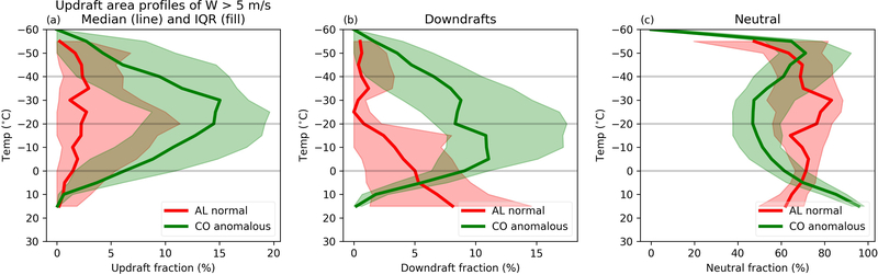
Microphysical and kinematic characteristics of two storm populations, based on their macroscale charge structures, are investigated in an effort to increase our understanding of the processes that lead to anomalous (or inverted charge) structures. Nine normal polarity cases (mid-level negative charge) with dual-Doppler and polarimetric coverage that occurred in northern Alabama, and six anomalous polarity cases (mid-level positive charge) that occurred in northeastern Colorado are included in this study. The results show that even though anomalous polarity storms formed in environments with similar instability, they had significantly larger and stronger updrafts. Moreover, the anomalous polarity storms evidently have more robust mixed-phase microphysics, based on a variety of metrics. Anomalous polarity storms in Colorado have much higher cloud base heights and shallower warm cloud depths in this study, leading us to hypothesize that anomalous polarity storms have lower amounts of dilution and entrainment. We infer positively charged graupel, and therefore high supercooled water contents, in the mid-levels of the anomalous storms based on the relationship between colocations of graupel and inferred positive charge from Lightning Mapping Array data. Using representative updraft speeds and warm cloud depths, the time required for a parcel to traverse from cloud base to the freezing level was estimated for each storm observation. We suggest this metric is the key discriminator between the two storm populations and leads us to hypothesize that it strongly influences the amount of supercooled water and the probability of positive charge in the midlevels, leading to an anomalous charge structure.

Figure 1:

Archetypal normal AL case study from 21 May 2012. (a) X-Z cross section of that case at 202341Z. Reflectivity values are shown in the color fill, following the colorbar on the right. Vectors show the U and W components of the wind, following the legend in the upper-right portion of the panel. Bilaterally smoothed two-dimensional LMA source density (within 1 km of the cross section) is shown in light contours. Each contour indicates 20%, 40%, 60%, 80%, and 100% of the maximum value for this case. Updraft speeds are shown in dark contours of 3, 5, 10, 20, and 30 m s⁻¹. A plan view of composite reflectivity is shown in the inset panel. The location of the X-Z cross section is illustrated by the black line. (b) Timeseries of vertical distribution of LMA source density (color fill), following the colorbar below the panel. The LMA modal height (green) follows the left axis, while the cell total flash rate (gray) following the right axis. (c) Timeseries of mean ice mass at each vertical level (color fill), following the colorbar below the panel. The mixed-phase 35 dBZ volume (gray) and the mixed-phase graupel volume (green) follow the right axis. The correlation coefficient between the vertical distributions of LMA source density and ice mass (gold dashed) follows the rightmost axis. (d) Timeseries of the 95^th percentile of updraft speed at each vertical level (color fill). Updraft volume > 5 m s⁻¹ (UV5) and > 10 m s⁻¹ (UV10) shown in the light and dark purple colors, respectively, and follow the right axis. The maximum updraft speed in the cell is shown in the dashed red line and follows the red axis on the far right. The time of the X-Z cross section and composite reflectivity is illustrated with a vertical line in panels b-d and the 0 °C, −20 °C and −40 °C levels are shown in dotted black lines in each panel.

Figure 2:

Similar to Figure 1 but for the archetypal anomalous CO case study from 06 June 2012. Note that dual-Doppler data is not available between 2230Z and 2236Z due to a temporary issue with the PAWNEE radar.

Figure 3:

(a) Vertical distribution of normalized LMA source densities for each normal AL storm, with temperature as the vertical coordinate. The red line indicates the −30 °C threshold bifurcating cells into normal or anomalous polarity. (b) Same as (a) but for each anomalous CO storm sample, red line indicates the −25 °C threshold. (c) Cumulative distribution of cell total flash rates for each storm sample.

Figure 4:

Distributions of (a) CAPE (J kg⁻¹), (b) NCAPE (m s⁻²), (c) LCL height (m AGL), (d) WCD (m), (e) adiabatic water content (g kg⁻¹), (f) precipitable water (mm), (g) surface temperature (C), (h) surface dew point (C), (i) average relative humidity (%) between 600–500 mb, (j) surface to 6 km shear (m s⁻¹), (k) CIN (J kg⁻¹), and (l) equilibrium height (m MSL) from attributed inflow soundings. The bars indicate the quantities associated with storm samples in this study. Median values of each quantity for both regions region and each study are indicated in each panel, in addition to the Spearman ranksum p value, which tests the null hypothesis by calculating the probability that both distributions are subsets of the same distribution.

Figure 5:

(a) Composite contoured frequency by altitude diagram (CFAD) for all normal AL storm samples, following the log-scale color bar below the panel. The lines indicate the average updraft (red) and downdraft (blue) for all normal AL cases. (b) Same as (a) but for the anomalous CO storm samples. (c) Cumulative distribution of the maximum W (measured by the 99^th percentile) for both storm populations. (d) Cumulative distributions of updraft volume greater than 5 m/s (UV5; solid line) and updraft volume greater than 10 m/s (UV10; dashed line) for both storm populations.

Figure 6:

(a) Median (line) and interquartile range (color fill) updraft area (W ≥ 5 m s⁻¹) for all storm samples at a particular temperature for each storm population. Converting radar heights to temperatures is done by interpolation using the attributed inflow sounding. (b) Same as (a) but for downdraft area (W < −3 m s⁻¹). (c) Same as (a) but for W between −3 and 5 m s⁻¹.

Figure 7:

(a) Fraction of total LMA sources collocated with a particular W bin at a particular height, averaged together for all normal AL storm samples. Contours show CFAD values of 1%, 10% and 30% of W. (b) Percentage of total LMA sources collocated with a particular bin of the horizontal gradient of W at a particular height for all normal AL storm samples. (c) Same as (a) but for the anomalous CO storm samples. (d) Same as (b) for the anomalous CO storm samples.

Figure 8:

Cumulative distributions of (a) mixed-phase graupel volume, (b) mixedphase 30 dBZ volume, (c) maximum graupel height (from inferred dominant hydrometeor type), (d) average mixed-phase graupel mass mixing ratio.

Figure 9:

(a) Mean vertical profile of radar reflectivity (VPRR) for each normal AL storm sample (light red lines) and the composite VPRR for the normal AL storm population (dark red line) and the composite VPRR for all anomalous CO storm population (dark green line). (b) Same as (a) but each thin green line is the mean VPRR for each individual anomalous CO storm sample. (c) Same as (a) but for max values instead of mean values in normal AL storm samples. (d) Same as (b) but for max values instead of mean values in anomalous CO storm samples.

Figure 10:

(a) Distributions of correlation coefficient between the vertical distribution of mean ice mass and the vertical distribution of LMA source density for every storm in both populations. (b) Same as (a) but correlations are computed between three-dimensional values of ice mass and LMA source density.

Figure 11:

(a) Estimates of warm cloud residence time for each population using different values of W. No particle fall speeds are included in the calculation of warm cloud residence times. (b) Same as (a) but assuming a constant 2 m s⁻¹ particle fall speed. (c) Same as (a) assuming a constant 4 m s⁻¹ particle fall speed. (d) Same as (a) assuming a constant 6 m s⁻¹ particle fall speed. If particle fall speed is greater than representative updraft speed, warm cloud residence time is set to 3600 s.

Figure 12:

Same as Figure 1, but for a normal polarity case in CO from 05 June 2012. VHF source distributions are not plotted from 2300Z to 2320Z because no lightning occurred within the cell during that time.

References

1. Albrecht RI, Morales CA, and Silva Dias MA (2011), Electrification of precipitating systems over the Amazon: Physical processes of thunderstorm development, Journal of Geophysical Research: Atmospheres, 116 (D8).
1. Atlas D, and Ulbrich CW (2000), An observationally based conceptual model of warm oceanic convective rain in the tropics, Journal of Applied Meteorology, 39 (12), 2165–2181.
1. Avila EE, and Pereyra RG (2000), Charge transfer during crystal-graupel collisions for two different cloud droplet size distributions, Geophys. Res. Lett, 27 (23), 3837–3840.
1. Baker MB, and Dash JG (1989), Charge transfer in thunderstorms and the surface melting of ice, J. Cry. Grow, 97, 770–776.
1. Barth M, and coauthors (2015), The Deep Clouds and Convective Chemistry (DC3) field campaign, Bull. Amer. Meteor. Soc
LinkOut - more resources