Multiscale higher-order TV operators for L1 regularization

Abstract

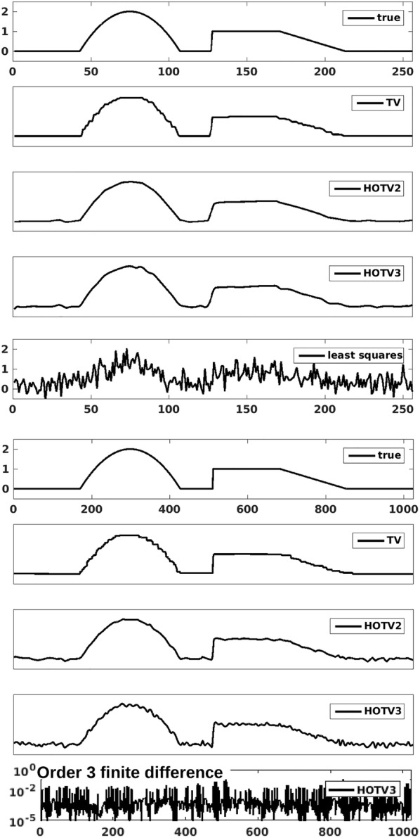
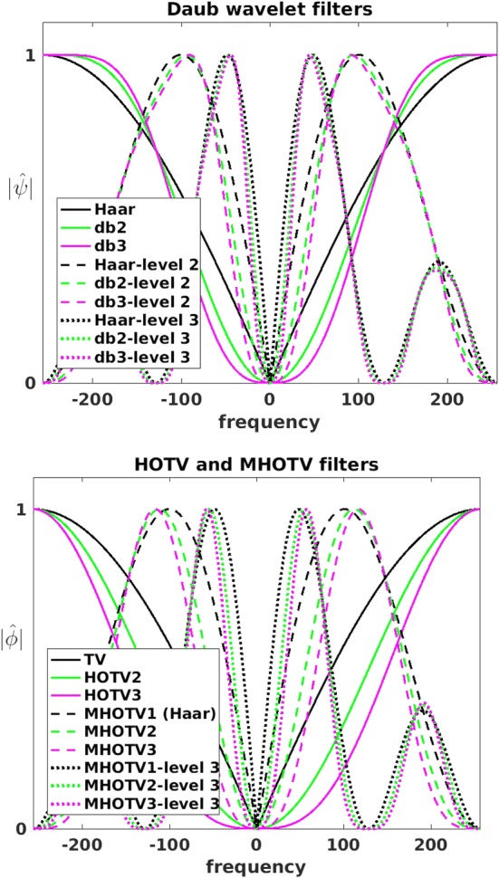
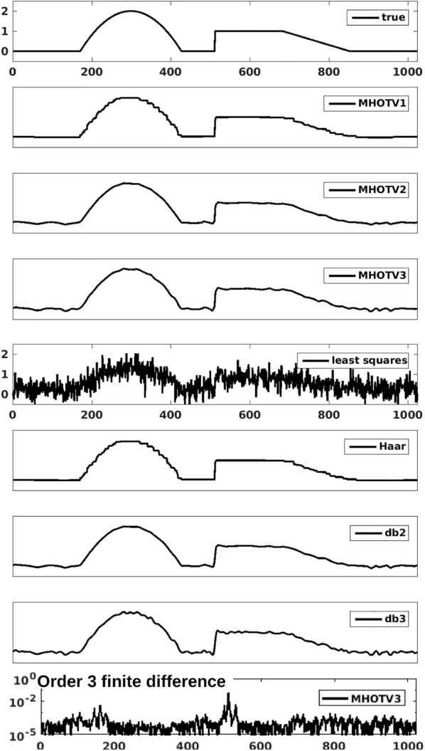
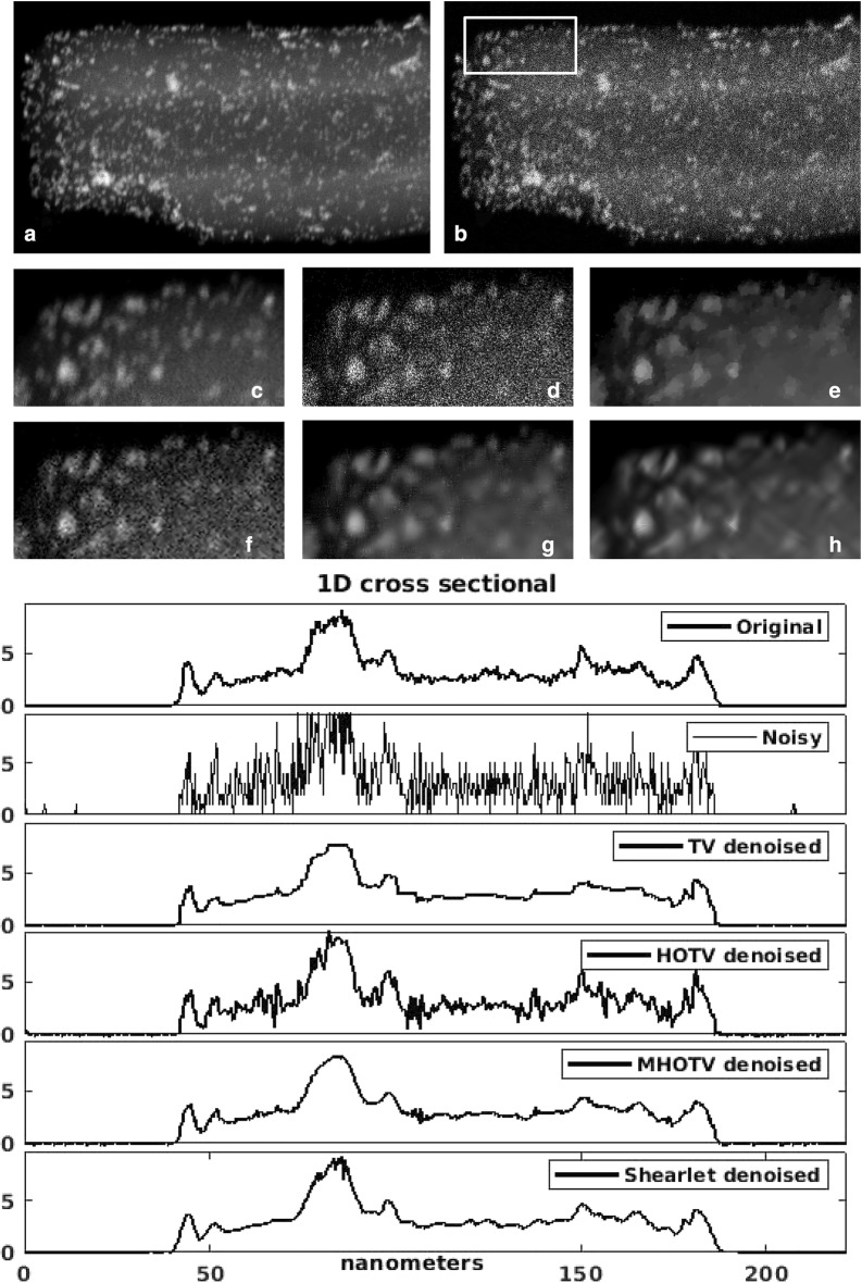
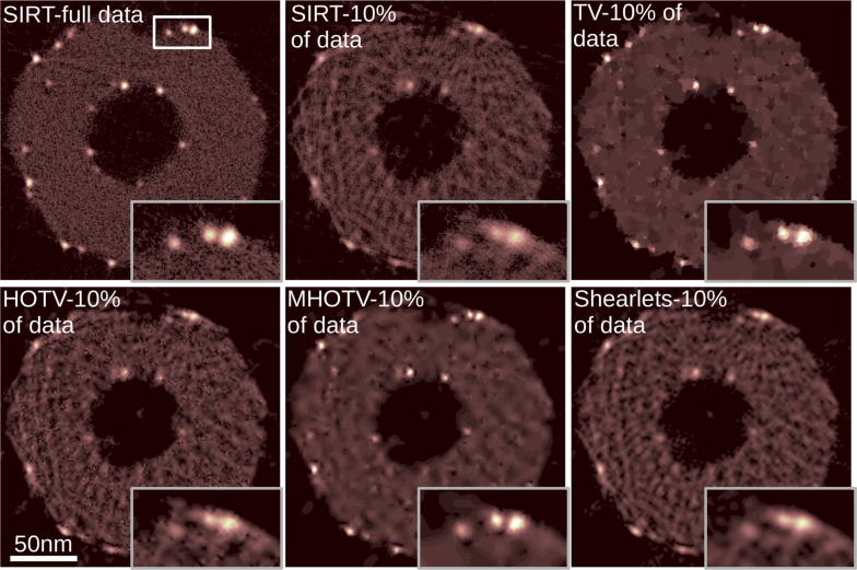
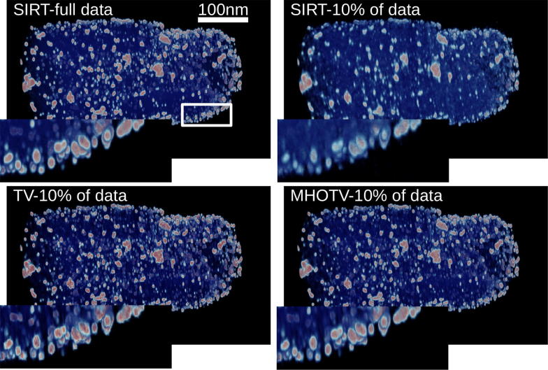
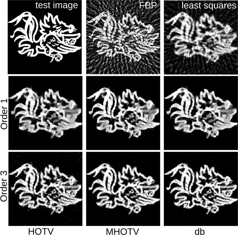
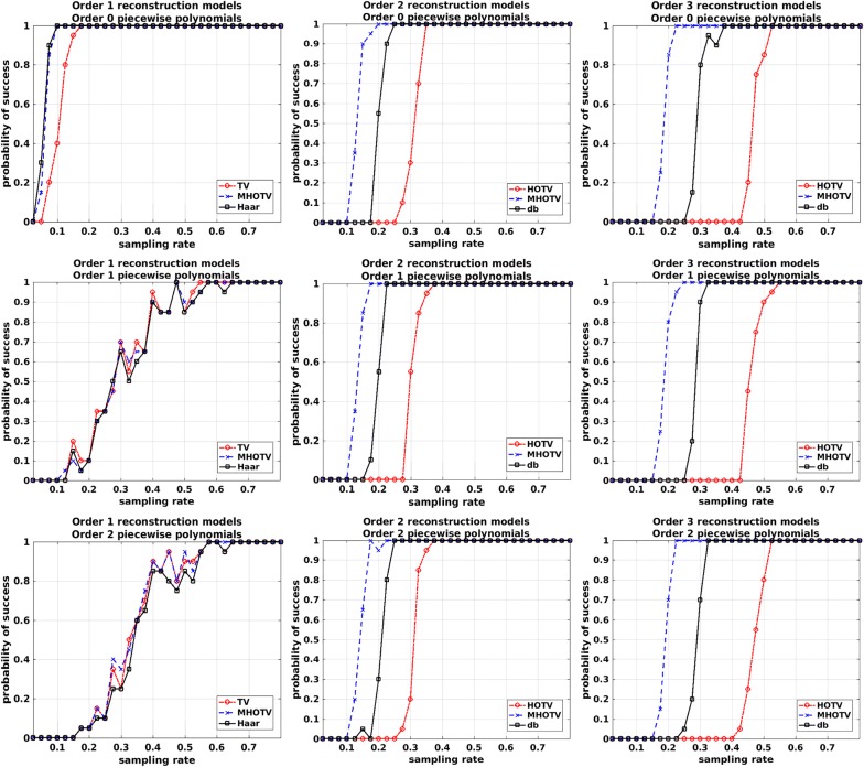
In the realm of signal and image denoising and reconstruction, ${\ell }_1$ regularization techniques have generated a great deal of attention with a multitude of variants. In this work, we demonstrate that the ${\ell }_1$ formulation can sometimes result in undesirable artifacts that are inconsistent with desired sparsity promoting ${\ell }_0$ properties that the ${\ell }_1$ formulation is intended to approximate. With this as our motivation, we develop a multiscale higher-order total variation (MHOTV) approach, which we show is related to the use of multiscale Daubechies wavelets. The relationship of higher-order regularization methods with wavelets, which we believe has generally gone unrecognized, is shown to hold in several numerical results, although notable improvements are seen with our approach over both wavelets and classical HOTV. These results are presented for 1D signals and 2D images, and we include several examples that highlight the potential of our approach for improving two- and three-dimensional electron microscopy imaging. In the development approach, we construct the tools necessary for MHOTV computations to be performed efficiently, via operator decomposition and alternatively converting the problem into Fourier space.

Keywords: ℓ 1 regularization; Electron tomography; Image reconstruction; Sparsity.

Fig. 1

Rows 2–4 and 7–9 reconstruction of a piecewise polynomial function of degree two shown in the top row over 256 (top 5 plots) and 1024 (bottom 5 plots) points from random sampling at 50%. The corresponding least squares solution is shown in the fifth plot, and the third-order finite difference of the HOTV3 solution over the 1024 grid is shown on the bottom

Fig. 2

The filters in Fourier space of wavelet and MHOTV convolution functions

Fig. 3

Reconstruction of a piecewise polynomial function of degree two over 1024 stencil from random sampling at 50%. Three scales are used for both the Daubechies wavelets and multiscale HOTV

Fig. 4

Denoising of an electron microscopy projection with Poisson noise. Small magnified patch is shown below for detailed analysis, where this patch is indicated in b. In a and c are the original image, with little noise, and in b and d are the simulated noisy images. In e is the TV denoised image, in f is the HOTV denoised, in g is the MHOTV denoised, and in h is the shearlet denoised by hard thresholding. One-dimensional plots of a single cross-section are shown on the right for an additional point of comparison

Fig. 5

The 2D tomographic reconstruction of a single cross section of the 3D object visualized by a 2D projection in Fig. 4. A small patch is magnified in the bottom right of each image, where this patch is indicated in the top left image. A total of 180 projections are available for the reconstruction (resulting in the reconstruction shown in the top left), and the remaining reconstructions shown are from limiting the data to only 18 projections, i.e., only 10% of the original data

Fig. 6

Shown is the volume rendering of the 3D tomographic reconstruction of the projected objected shown in Fig. 4. A small patch is magnified in the bottom left of each image, where this patch is indicated in the top left image. A total of 180 projections are available for the reconstruction (resulting in the reconstruction shown in the top left), and the remaining reconstructions shown are from limiting the data to only 18 projections, i.e., only 10% of the original data

Fig. 7

Reconstructions of phantom image from 29 tomographic projections. Orders 1 and 3 are shown for the regularization approaches. In the top right are the least squares and filtered backprojection (FBP) reconstructions for a baseline comparison

Fig. 8

Probability of success for HOTV, MHOTV, and Daubechies wavelets at orders 1 (left column), 2 (middle column) and 3 (right column). A successful recovery is deemed whenever the relative ${\ell }_2$ error between the reconstruction and the true signal is less than ${10}^{-2}$. Top row: piecewise constant functions. Middle row: piecewise linear functions. Bottom row: piecewise quadratic functions

References

1. Rudin LI, Osher S, Fatemi E. Nonlinear total variation based noise removal algorithms. Physica D Nonlinear Phenomena. 1992;60(1):259–268. doi: 10.1016/0167-2789(92)90242-F. - DOI
1. Wei S-J, Zhang X-L, Shi J, Xiang G. Sparse reconstruction for SAR imaging based on compressed sensing. Prog Electromagn Res. 2010;109:63–81. doi: 10.2528/PIER10080805. - DOI
1. Bhattacharya, S., Blumensath, T., Mulgrew, B., Davies, M.: Fast encoding of synthetic aperture radar raw data using compressed sensing. In: IEEE 2007 IEEE/SP 14th workshop on statistical signal processing, pp. 448–452 (2007)
1. Lustig M, Donoho D, Pauly JM. Sparse MRI: the application of compressed sensing for rapid MR imaging. Magn. Resonance Med. 2007;58(6):1182–1195. doi: 10.1002/mrm.21391. - DOI - PubMed
1. Lysaker M, Lundervold A, Tai X-C. Noise removal using fourth-order partial differential equation with applications to medical magnetic resonance images in space and time. IEEE Trans. Image Process. 2003;12(12):1579–1590. doi: 10.1109/TIP.2003.819229. - DOI - PubMed
LinkOut - more resources