. 2018 Nov 12;14(11):e1006535.
doi: 10.1371/journal.pcbi.1006535. eCollection 2018 Nov.

Visual physiology of the layer 4 cortical circuit in silico

Affiliations

Visual physiology of the layer 4 cortical circuit in silico

Anton Arkhipov et al. PLoS Comput Biol. .

Abstract

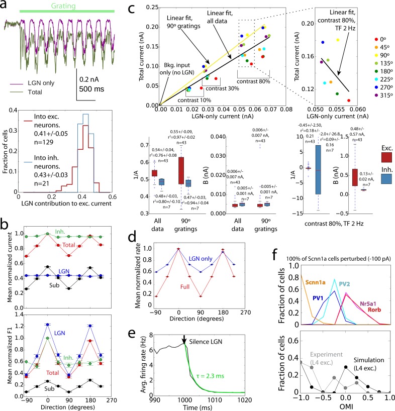
Despite advances in experimental techniques and accumulation of large datasets concerning the composition and properties of the cortex, quantitative modeling of cortical circuits under in-vivo-like conditions remains challenging. Here we report and publicly release a biophysically detailed circuit model of layer 4 in the mouse primary visual cortex, receiving thalamo-cortical visual inputs. The 45,000-neuron model was subjected to a battery of visual stimuli, and results were compared to published work and new in vivo experiments. Simulations reproduced a variety of observations, including effects of optogenetic perturbations. Critical to the agreement between responses in silico and in vivo were the rules of functional synaptic connectivity between neurons. Interestingly, after extreme simplification the model still performed satisfactorily on many measurements, although quantitative agreement with experiments suffered. These results emphasize the importance of functional rules of cortical wiring and enable a next generation of data-driven models of in vivo neural activity and computations.


Conflict of interest statement

The authors have declared that no competing interests exist.

Figures

Fig 1
Fig 1. Construction of the model.
(a) The biophysical and LIF portions of the model on the cortical surface with delineations of cortical areas (top; “VISp” is V1; the other labels starting with “VIS” correspond to higher visual areas) and with individual cells rendered (bottom; only a small subset of cells is shown for clarity). (b) Morphologies and action potential shapes of the five neuron models used to generate the L4 network; numbers of cells of each type are listed. (c-e) Connection probability (c,d) and synaptic weights (e) of excitatory (E) or inhibitory (I) cell targets and sources. The rules incorporate the dependence on the distance between somata (c) or difference of the assigned preferred orientations, Δori (d, e). Rules dependent on Δori were applied to E-to-E connections only, and synaptic weights for all connections were independent of distance. (f) Connection probability computed for cells within 50 μm using actual preferred orientation observed in simulations (cf. [24]). Numbers of connected and total pairs, used to obtain the probability, are shown inside the bars. (g) Three types of LGN filters (ON, OFF, and ON/OFF), superimposed onto an image, providing inputs to a L4 cell. Example filter’s spatial and temporal profiles are at the bottom. (h) The proportion of excitatory thalamocortical synapses (VGLUT2+) in the neuropil of V1 L4, as determined experimentally using EM. Proportions for individual samples of tissue are in gray; mean and s.e.m. for each mouse are in black. Right, an exemplar EM image of a putative VGLUT2+ synapse from the LGN onto an L4 neuron (Sp, spine; Bt, bouton; arrows: postsynaptic densities within the spine).
Fig 2
Fig 2. Examples of simulated responses to various visual stimuli.
(a) Spontaneous activity in the model was generated by waves of background excitation (“Bkg. on”, yellow arrow denotes the direction of motion of the yellow bar-like region) alternated with intervals of no background excitation (“Bkg. off”). (b) Model activity in a gray screen trial. Examples of membrane potential traces from simulated biophysical cells are in the middle. (c) Spike raster in response to a drifting grating (TF = 4 Hz, at 0 degrees direction). Bottom, example orientation tuning curves for an excitatory and inhibitory cell from simulation. (d) Spikes in response to a 50 ms full-field flash. (e) Spike raster for a single trial of a natural movie (top) and for a temporally scrambled version of the same movie (bottom). The raster in (b) shows all neurons and those in (c-e) for clarity show the 10,000 cells in the biophysical core of the model (inset on top of (c) zooms in on 200 cells). All rasters are examples from one trial; all trials used unique combinations of “Bkg. on” and “Bkg. off” states (shown at the bottom of plots), which overlapped (or not) in different ways with the visual stimuli.
Fig 3
Fig 3. Benchmarking the simulation results.
(a) Log-normal like distribution of firing rates. Top, firing rates of all biophysical cells from three models during spontaneous activity and in response to a drifting grating, averaged over 10 trials. Large red dots are firing rates averaged over all cells in 0.1 Hz bins over the spontaneous activity axis. Bottom, examples of firing rate distributions on a log scale for a single trial. Solid lines indicate log-normal fits of the data. (b) Comparison of the spontaneous rates, maximal rates in response to gratings (Rmax), orientation selectivity index (OSI), and direction selectivity index (DSI) between the simulation (by cell type, color) and experimental measurements using extracellular electrophysiology (gray). Here and in all other box plots, the box bottom and top mark the inter-quartile range (IQR), the median is in red, whiskers mark +/-1.5 IQR; mean and standard deviation are shown in black (see Methods for further details). “An.”–experiments in anesthetized mice, “Aw.”–in awake mice. (c) The local field potential (LFP; see Methods) measured at the center of the L4 model, for a drifting grating. The spectra from 10 trials are shown in gray, and the averaged spectrum is in black. (d) The model PSTH in response to a 50 ms flash (average over all biophysical excitatory cells, all models, and all trials, in 2 ms bins). (e) The magnitude and time-to-peak (from flash onset) for the first and second peaks of the response to the 50 ms flash, for both simulation and electrophysiological data. (f) Distributions of lifetime sparsity of simulated and experimental responses of excitatory neurons, computed for three directions of a grating (0, 45, and 90 degrees) and for three movies. See Methods for details on computing all values presented.
Fig 4
Fig 4. Mechanistic characterization of the model.
(a) Cortical amplification of the LGN inputs. The excitatory currents (from the LGN only, as well as total) in biophysical cells were measured using voltage clamp recordings. Top–an example; bottom–distributions of LGN contribution to the total excitatory current across excitatory and inhibitory cells (computed for each cell as the average current over time and over all trials of the preferred orientation). (b) Tuning curves for the mean and F1 component of the total and LGN-only currents, and their difference (“Sub”, i.e., the cortical component), as well as inhibitory current. The data for each cell were normalized to the peak value of the “Total” and shifted so that the preferred direction is at 0 degrees; averages and s.e.m. over all recorded excitatory cells are shown (TF = 2 Hz, contrast 80%). The inhibitory currents were normalized and aligned to their own peak values, since their magnitude is significantly higher than that of excitatory currents. (c) Amplification of excitatory current. Top, the total current vs. the LGN-only current, for an individual Rorb cell (each point is an average over time and over 10 trials). Linear fits (Itot = A ILGN + B) are shown for data aggregated from all grating directions, TFs, and contrasts (black), for one selected direction (yellow), and for a fixed contrast and TF (i.e., representing a sample direction tuning curve; right plot). Bottom, summary of linear fits across all cells analyzed. (d) Tuning curves for mean firing rate in full network simulations (“Full”, red) and in simulations where all connections except the feedforward connections from the LGN were removed (“LGN only”, blue). The data for each cell were normalized to the peak value of the “Full” and shifted so that the preferred direction is at 0 degrees; averages and s.e.m. over all excitatory cells are shown (TF = 2 Hz, contrast 80%). (e) Simulations of responses to a drifting grating, with the LGN activity switched off at 1000 ms. The black curve is the firing rate averaged over all cells, models, and trials; green is the exponential fit. (f) Distribution of the optogenetic modulation index (OMI) by cell type in responses to gratings, for simulations of optogenetic silencing of the Scnn1a population (top). Combined distribution for all biophysical excitatory cells is compared to the experimental result (bottom).
Fig 5
Fig 5. Like-to-like vs. random connectivity and synaptic weights.
(a) Distribution of OSI for biophysical excitatory cells for the LL, RL, LR, and RR cases. (b) Tuning curves for the mean total and LGN-only currents, and their difference (“Sub”, i.e., the cortical component). The data for each cell were normalized to the peak value of the “Total” and shifted so that the preferred direction is at 0 degrees; averages and s.e.m. over all recorded excitatory cells are shown (TF = 2 Hz, contrast 80%).
Fig 6
Fig 6. Comparison of biophysical and all-LIF simulations employing the IntFire1 or IntFire4 models.
(a) An example spike raster in response to a drifting grating in an all-LIF IntFire1 simulation. (b) Spontaneous rate, Rmax, OSI and DSI by cell type. (c) Spectra of multi-unit activity (weighted by 1/r, where r is the distance from the cell to the center of the system). This is used as a proxy to LFP, which cannot be directly computed for the point-neuron models. Note that exact match between this metric and the actual LFP computed for biophysical model (see Fig 3C) is not expected, but they both exhibit similar features, such as a prominent peak at ~20 Hz. (d) Distributions of lifetime sparsity of responses to gratings and movies, averaged over 10 trials. The data are for three directions of a grating (0, 45, and 90 degrees) and for three movies. (e) Distributions of LGN contribution to the total excitatory synaptic inputs across excitatory and inhibitory cells (in the IntFire1 and IntFire4 cases, this is computed for each cell as the average synaptic input over time and over all trials of the preferred orientation; see Methods), for TF = 2 Hz drifting gratings. (f) Distribution of OSI for excitatory cells for the LL, RL, LR, and RR cases.
Fig 7
Fig 7. LGN filters.
(a) Example responses of a single filter to visual stimuli, as a time-dependent firing rate that is the filter output (blue) and the firing rate computed from generated spike trains, averaged over all trials (green). The panel for images contains responses to 10 images shown in a sequence, 250 ms each. (b) F0 and F1 components of the responses to gratings for two example LGN filters. Tuning curves to orientation, SF, and TF are shown. The data points are averages from generated spike trains over time and over trials. (c) Connecting LGN filters to L4 cells. Geometry in the visual space is illustrated. The left panel shows centers of all filters present in a portion of the visual space around the mapped position of an example excitatory cell from L4. The dashed lines correspond to the “lasso” subfields around one illustrative L4 cell, used to capture input LGN filters of the ON, OFF, and ON/OFF type. The filters that are selected to send inputs to this L4 cells are in deep color; all other filters are dimmed. On the right, the same L4 cell with the filters selected to provide inputs to it are shown. For the filters, the approximate size of their receptive subfields is illustrated (a single subfield for ON or OFF filters and two subfields for ON/OFF filters; the radius of each RF circle is 2σC). (d) Convergence of LGN connectivity onto L4 cells that are not connected to each other (“No con.”), one-way connected (“One-way con.”), and reciprocally connected (“Reciprocal con.”). For each pair of L4 cells, the LGN convergence is defined as the number of LGN filters that connect to both cells divided by the sum of the numbers of LGN filters connected to each of the cells. The data are aggregated from three L4 models.

References

    1. California Institute of Technology. Caltech Library Archives [Internet]. Available from: http://archives-dc.library.caltech.edu/islandora/object/ct1:483
    1. Markram H. et al. Reconstruction and Simulation of Neocortical Microcircuitry. Cell 163, 456–492 (2015). 10.1016/j.cell.2015.09.029 - DOI - PubMed
    1. Traub R.D. et al. Single-column thalamocortical network model exhibiting gamma oscillations, sleep spindles, and epileptogenic bursts. J. Neurophysiol. 93, 2194–2232 (2005). 10.1152/jn.00983.2004 - DOI - PubMed
    1. Zhu W, Shelley M, and Shapley R. A neuronal network model of primary visual cortex explains spatial frequency selectivity. J. Comput. Neurosci. 26, 271–287 (2009). 10.1007/s10827-008-0110-x - DOI - PubMed
    1. Buzsaki G., and Mizuseki K. The log-dynamic brain: how skewed distributions affect network operations. Nat Rev Neurosci. 15, 264–278 (2014). 10.1038/nrn3687 - DOI - PMC - PubMed

Publication types

LinkOut - more resources