Comparing Bayesian and non-Bayesian accounts of human confidence reports

Abstract

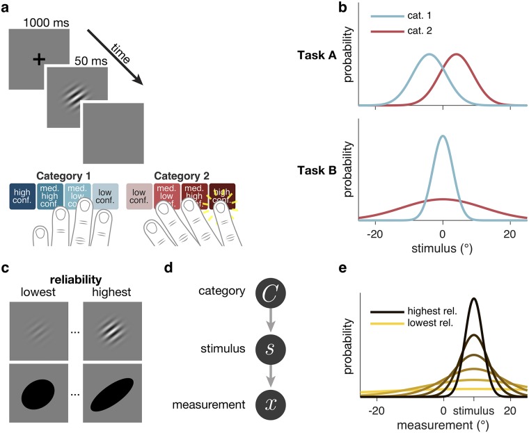
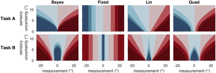
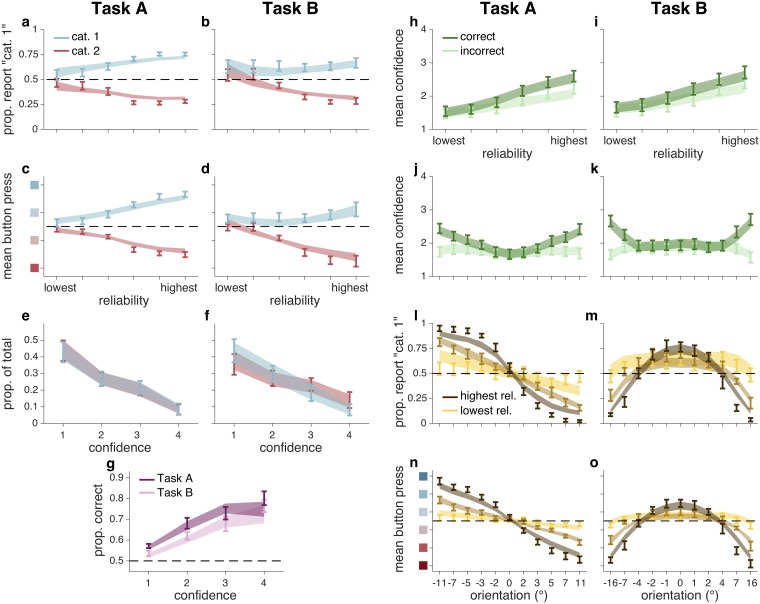
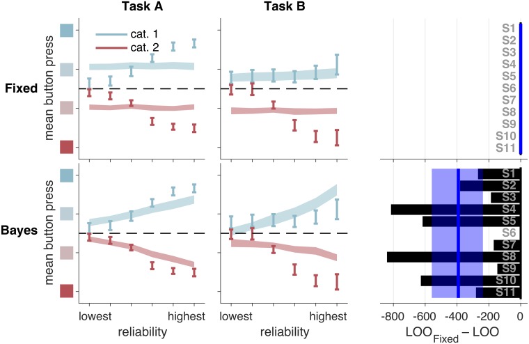
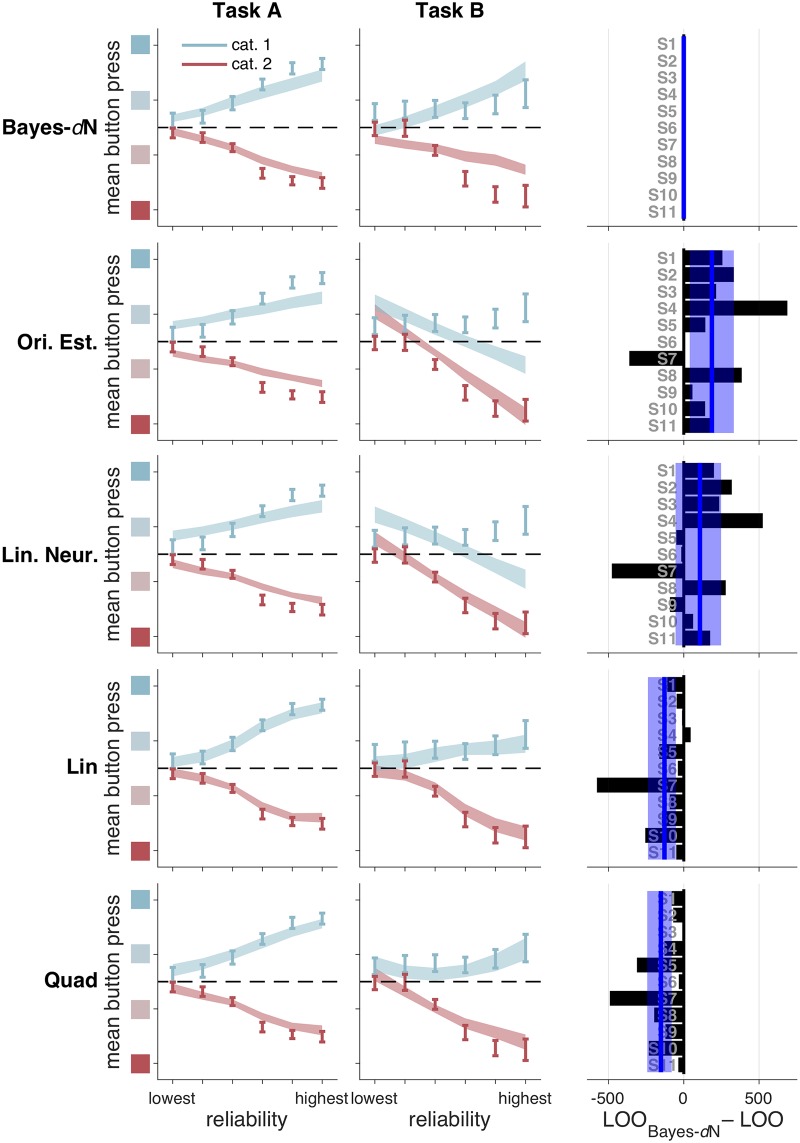
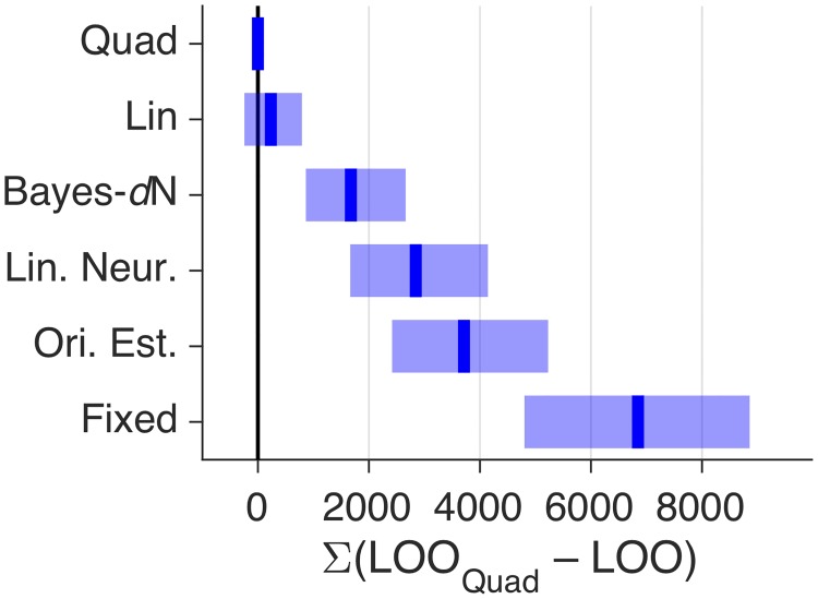
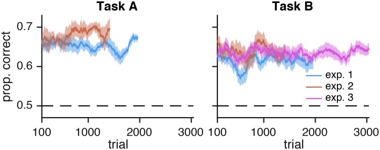
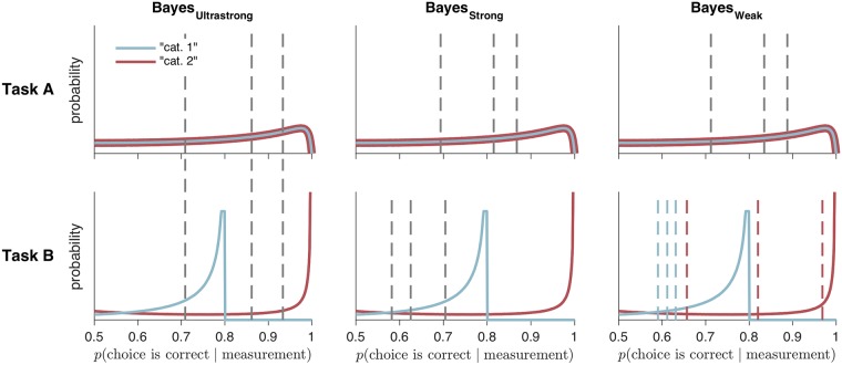
Humans can meaningfully report their confidence in a perceptual or cognitive decision. It is widely believed that these reports reflect the Bayesian probability that the decision is correct, but this hypothesis has not been rigorously tested against non-Bayesian alternatives. We use two perceptual categorization tasks in which Bayesian confidence reporting requires subjects to take sensory uncertainty into account in a specific way. We find that subjects do take sensory uncertainty into account when reporting confidence, suggesting that brain areas involved in reporting confidence can access low-level representations of sensory uncertainty, a prerequisite of Bayesian inference. However, behavior is not fully consistent with the Bayesian hypothesis and is better described by simple heuristic models that use uncertainty in a non-Bayesian way. Both conclusions are robust to changes in the uncertainty manipulation, task, response modality, model comparison metric, and additional flexibility in the Bayesian model. Our results suggest that adhering to a rational account of confidence behavior may require incorporating implementational constraints.

Fig 1. Task design.

(a) Schematic of a test block trial. After stimulus offset, subjects reported category and confidence level with a single button press. (b) Stimulus distributions for Tasks A and B. (c) Examples of low and high reliability stimuli. Six (out of eleven) subjects saw drifting Gabors, and five subjects saw ellipses. (d) Generative model. (e) Example measurement distributions at different reliability levels. In all models (except Linear Neural), the measurement is assumed to be drawn from a Gaussian distribution centered on the true stimulus, with s.d. dependent on reliability.

Fig 2. Decision rules/mappings in four models.

Each model corresponds to a different mapping from a measurement and uncertainty level to a category and confidence response. Colors correspond to category and confidence response, as in Fig 1a. Plots were generated using parameter values that were roughly similar to those found after fitting subject data but were chosen primarily to illustrate the different features of the models.

Fig 3. Behavioral data and fits from best model (Quad), experiment 1.

Error bars represent ±1 s.e.m. across 11 subjects. Shaded regions represent ±1 s.e.m. on model fits. (a,b) Proportion “category 1” reports as a function of stimulus reliability and true category. (c,d) Mean button press as a function of stimulus reliability and true category. (e,f) Normalized histogram of confidence reports for both true categories. (g) Proportion correct category reports as a function of confidence report and task. (h,i) Mean confidence as a function of stimulus reliability and correctness. (j,k) Mean confidence as a function of stimulus orientation and reliability. (l,m) Proportion “category 1” reports as a function of stimulus orientation and reliability. (n,o) Mean button press as a function of stimulus orientation and reliability. (c,d,n,o) Vertical axis label colors correspond to button presses, as in Fig 1a. (l–o) For clarity, only 3 of 6 reliability levels are shown, although models were fit to all reliability levels.

Fig 4. Model fits and model comparison for models Fixed and Bayes.

Bayes provides a better fit, but both models have large deviations from the data. Left and middle columns: model fits to mean button press as a function of reliability, true category, and task. Error bars represent ±1 s.e.m. across 11 subjects. Shaded regions represent ±1 s.e.m. on model fits, with each model on a separate row. Right column: LOO model comparison. Bars represent individual subject LOO scores for Bayes, relative to Fixed. Negative (leftward) values indicate that, for that subject, Bayes had a higher (better) LOO score than Fixed. Blue lines and shaded regions represent, respectively, medians and 95% CI of bootstrapped mean LOO differences across subjects. These values are equal to the summed LOO differences reported in the text divided by the number of subjects. Although we plot data as a function of the true category here, the model only takes in measurement and reliability as an input; it is not free to treat individual trials from each true category differently.

Fig 5. Model fits and model comparison for Bayes-dN and heuristic models.

In both tasks, Bayes-dN fails to describe the data at high reliabilities; Lin and Quad provides a good fit at most reliabilities. Left and middle columns: as in Fig 4. Right column: bars represent individual subject LOO scores for each model, relative to Bayes-dN. Negative (leftward) values indicate that, for that subject, the model in the corresponding row had a higher (better) LOO score than Bayes-dN. Blue lines and shaded regions: as in Fig 4.

Fig 6. Comparison of core models, experiment 1.

Models were fit jointly to Task A and B category and confidence responses. Blue lines and shaded regions represent, respectively, medians and 95% CI of bootstrapped summed LOO differences across subjects. LOO differences for these and other models are shown in S1a Fig.

Fig 7

(a) In experiment 1, Task B, on trials in which the subject chose category 2, mean confidence increases with the absolute value of stimulus orientation. (b) The “positive evidence” in favor of category 2, however, decreases with the absolute value of stimulus orientation. This plot depicts the category-conditioned stimulus distribution p(s ∣ C = 2); positive evidence in this experiment is equivalent to the likelihood p(x ∣ C = 2), which is just p(s ∣ C = 2) convolved with the subject’s measurement noise.

Fig 8. Performance as a function of number of trials, for both tasks and for all experiments.

Performance was computed as a moving average over test trials (200 trials wide). Shaded regions represent ±1 s.e.m. over subjects. Performance did not change significantly over the course of each experiment.

Fig 9. Distributions of posterior probabilities of being correct, with confidence criteria for Bayesian models with three different levels of strength.

Solid lines represent the distributions of posterior probabilities for each category and task in the absence of measurement noise and sensory uncertainty. Dashed lines represent confidence criteria, generated from the mean of subject 4’s posterior distribution over parameters. Each model has a different number of sets of mappings between posterior probability and confidence report. In Bayes_Ultrastrong, there is one set of mappings. In Bayes_Strong, there is one set for Task A, and another for Task B. In Bayes_Weak, as in the non-Bayesian models, there is one set for Task A, and one set for each reported category in Task B. Plots were generated from the mean of subject 4’s posterior distribution over parameters as in Fig 2.

Fig 10. Posterior distributions over parameter values for an example model.

Each subplot represents a parameter of the model. Each colored histogram represents the sampled posterior distribution for a parameter and a subject in experiment 1, with colors consistent for each subject. The limits of the x-axis indicates the allowable range for each parameter. Black triangles indicate the overall mean parameter value.

Fig 11. Example analysis of a bootstrapped confidence interval.

(a) Uncertainty estimates for bootstrapped confidence intervals, as a function of the number of subjects included. Blue line represents the median bootstrapped mean of LOO differences, and black lines indicate the lower and upper bounds of the 95% CI. Error bars represent ±1 s.d. (b) For comparison to a, the standard style of plot used to show model comparison results (e.g., Fig 4).

Fig 12. Model recovery analysis.

Shade represents the difference between the mean AIC score (across datasets) for each fitted model and for the one with the lowest mean AIC score. White squares indicate the model that had the lowest mean AIC score when fitted to data generated from each model. The squares on the diagonal indicate that the true generating model was the best-fitting model, on average, in all cases.

References

1. Meyniel F, Sigman M, Mainen ZF. Confidence as Bayesian probability: From neural origins to behavior. Neuron. 2015. October;88(1):78–92. 10.1016/j.neuron.2015.09.039 - DOI - PubMed
1. Brown AS. A review of the tip-of-the-tongue experience. Psychol Bull. 1991. March;109(2):204–223. 10.1037/0033-2909.109.2.204 - DOI - PubMed
1. Persaud N, McLeod P, Cowey A. Post-decision wagering objectively measures awareness. Nat Neurosci. 2007. January;10(2):257–261. 10.1038/nn1840 - DOI - PubMed
1. Bahrami B, Olsen K, Latham PE, Roepstorff A. Optimally interacting minds. Science. 2010;329(5995):1081–1085. 10.1126/science.1185718 - DOI - PMC - PubMed
1. Fleming SM, Weil RS, Nagy Z, Dolan RJ, Rees G. Relating introspective accuracy to individual differences in brain structure. Science. 2010. September;329(5998):1541–1543. 10.1126/science.1191883 - DOI - PMC - PubMed
Publication types