Microtubule Feedback and LET-99-Dependent Control of Pulling Forces Ensure Robust Spindle Position

Abstract

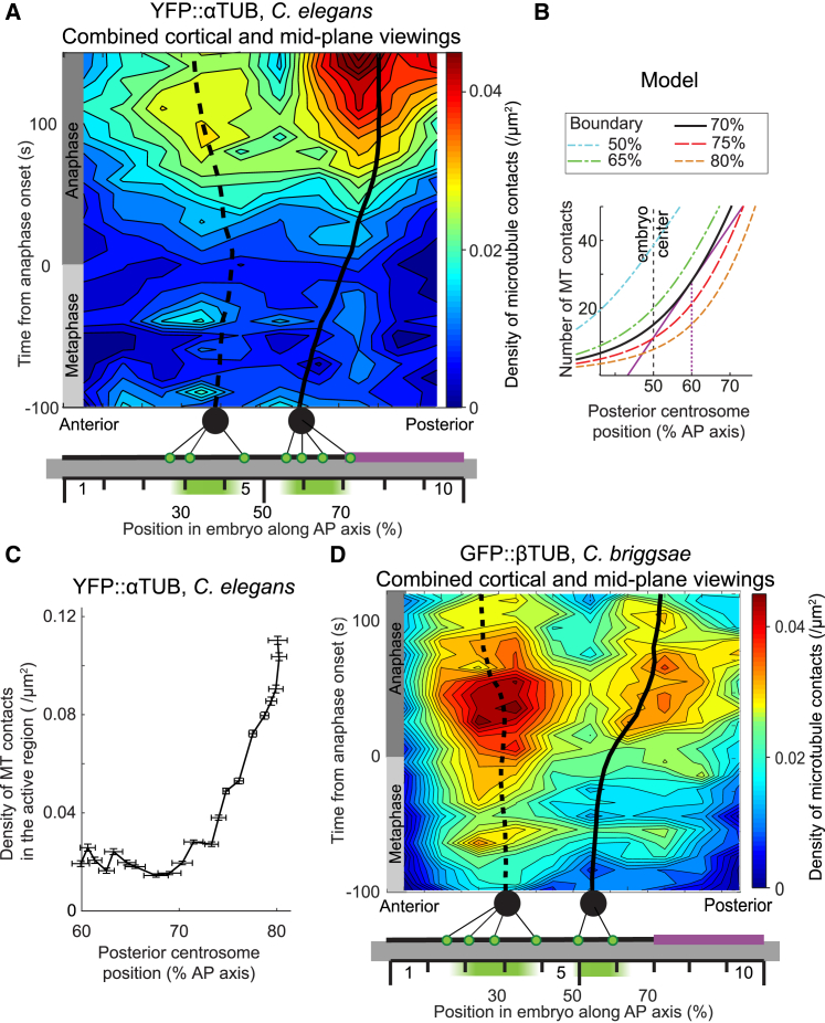
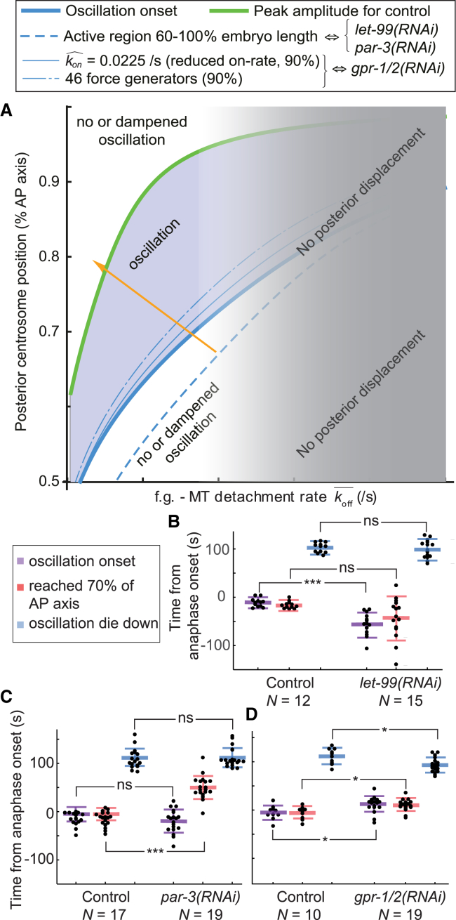
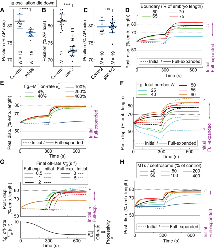
During asymmetric division of the Caenorhabditis elegans zygote, to properly distribute cell fate determinants, the mitotic spindle is asymmetrically localized by a combination of centering and cortical-pulling microtubule-mediated forces, the dynamics of the latter being regulated by mitotic progression. Here, we show a, to our knowledge, novel and additional regulation of these forces by spindle position itself. For that, we observed the onset of transverse spindle oscillations, which reflects the burst of anaphase pulling forces. After delaying anaphase onset, we found that the position at which the spindle starts to oscillate was unchanged compared to control embryos and uncorrelated to anaphase onset. In mapping the cortical microtubule dynamics, we measured a steep increase in microtubule contact density after the posterior centrosome reached the critical position of 70% of embryo length, strongly suggesting the presence of a positional switch for spindle oscillations. Expanding a previous model based on a force-generator temporal control, we implemented this positional switch and observed that the large increase in microtubule density accounted for the pulling force burst. Thus, we propose that the spindle position influences the cortical availability of microtubules on which the active force generators, controlled by cell cycle progression, can pull. Importantly, we found that this positional control relies on the polarity-dependent LET-99 cortical band, the boundary of which could be probed by microtubules. This dual positional and temporal control well accounted for our observation that the oscillation onset position resists changes in cellular geometry and moderate variations in the active force generator number. Finally, our model suggests that spindle position at mitosis end is more sensitive to the polarity factor LET-99, which restricts the region of active force generators to a posterior-most region, than to microtubule number or force generator number/activity. Overall, we show that robustness in spindle positioning originates in cell mechanics rather than biochemical networks.

Figure 1

Microtubule contact density at the cell cortex. (A–C) Exemplar spinning disk micrographs of C. elegans at the cortical plane with YFP::α-tubulin labeling of microtubules, viewed at 10 frames per second. The posterior tip of the embryo is on the right side of the pictures. The raw image (A) was denoised (B) using the Kalman filter, and microtubule contacts were tracked (C, green lines) using the u-track algorithm with the parameters listed in Table S3. The scale bar represents 10 μm. (D) The experimental setup for viewing microtubule contact density at the cell cortex. The scale represents the 10 regions along the anteroposterior (AP) axis used for analysis (Materials and Methods). Red and blue disks represent the anterior and posterior centrosomes, respectively, and the light blue clouds are the chromosomes. Microtubules emanating from the centrosomes are exemplified using thin black lines. The posterior-most crescent where the active force generators are located (the so-called active region) corresponds to the purple cortical region. (E) A semi-log plot of the histogram of the microtubule contact durations at the cortex during metaphase and anaphase for a single embryo (black dots), fitted with an exponential decay (gray line) corresponding to a characteristic time of 0.95 ± 0.03 s (N = 3832 microtubule contacts). (F and G) Microtubule contact densities at the cortex obtained by analyzing spinning disk microscopy images of (F) the YFP::α-tubulin-labeled microtubule strain in N = 12 C. elegans embryos and (G) the GFP::β-tubulin-labeled microtubule strain in N = 8 C. briggsae embryos. Microtubule contact densities measured at 23°C for each embryo were then averaged along the AP axis within 10 regions of equal width and over a 10-s running time window, and finally the average over embryos was computed (Materials and Methods).

Figure 2

Astral microtubules preferentially contact the cortex in the area closest to the centrosomes. (A) Microtubule contact density at the cell cortex in C. elegans with superposed centrosome trajectories obtained by combining two data sets. First, the densities, shown here as an interpolated heat map, were measured in the microtubule-labeled strain at the cortex and obtained by averaging the densities along the AP axis within 10 regions of equal width and over a 10-s running time window, finally taking the mean over embryos (Materials and Methods). Data are the same as in Fig. 1F. Second, the average trajectories of the centrosomes were obtained by imaging the same strain at the spindle plane (N = 8 embryos) and superposing the results on the microtubule-contact-density map. The dashed line represents the anterior centrosome trajectory, and the solid line indicates the posterior one. At the bottom is a schematic of the experimental setup in which centrosomes are shown as black disks, with thin black lines depicting the astral microtubules. Microtubule contacts at the cortex are shown as green dots. The active region, which is used to compute (C), corresponds to the purple cortical horizontal line. (B) The modeled number of microtubules contacting the cortex in the active region versus the posterior displacement of the centrosome along the AP axis, with the active region boundary expressed as a percentage of embryo length. The thick black line corresponds to a boundary at 70%, mimicking the untreated embryo. In this case, the number of contacts started to increase steeply at a position above 60% (purple line). Blue and green curves model let-99(RNAi) or par-3(RNAi) experiments in which the boundary was displaced anteriorly. Red and orange curves show the cases of posteriorly displaced boundaries. (C) The density of microtubule contacts versus the position of the posterior centrosome in a region ranging from 70 to 100% of the AP axis, computed from the data shown in (A). (D) The microtubule contact density at the cortex in C. briggsae with superposed centrosome trajectories represented similarly to (A). Microtubule contact densities at the cortex were obtained by viewing a GFP::β-tubulin-labeled microtubule strain. The data are the same as in Fig. 1 G. Centrosome trajectories were obtained in a second experiment by imaging a GFP::γ-tubulin;GFP::HIS-11-labeled centrosome and histone strain (N = 7 C. briggsae embryos) at the spindle plane.

Figure 3

Expanded model accounts for positional and temporal regulations of cortical forces. (A) Schematics of the expanded model highlighting the players (top row), the quantity they regulate (second row), how they control forces (module, third row), and some related phenotypes (bottom row). Pink/yellow colors correspond to the positional control involving astral microtubule dynamics and the active region created by LET-99, and blue depicts the time control involving force generator dynamics. Although both controls participate in oscillation onset (purple), final spindle position mostly depends on active region extent (yellow) and oscillation die down on time control (blue). (B) The modeled number of engaged force generators versus the posterior displacement of the centrosome along the AP axis, with the active region boundary expressed as a percentage of embryo length. The thick black line represents the case in which active region boundary is located at 70% of the AP axis, mimicking the control embryo. Blue and green curves model let-99(RNAi) and par-3(RNAi) experiments in which the boundary was displaced anteriorly. Red and orange curves show cases of posteriorly displaced boundaries. Gray shading indicates when the number of engaged force generators is too low to permit oscillation. The parameters used are listed in Table S1. (C and D) Positions of the posterior centrosome at oscillation onset (C) in let-99(RNAi) (N = 15) and control (N = 12) embryos and (D) in par-3(RNAi) (N = 19) and control (N = 17) embryos, with centrosomes labeled by GFP::γ-tubulin. Bee swarm plots report values obtained for each embryo. Large thick horizontal bars depict the mean, whereas error bars indicate SD and asterisks indicate significant differences (Materials and Methods).

Figure 4

Embryo length has less effect on oscillation onset position than on its timing. (A) The modeled number of engaged force generators versus the posterior displacement of the centrosome along the AP axis as a percentage of embryo length. The line colors indicate the embryo length: untreated embryos are black; the shorter embryos corresponding to those produced by cid-1(RNAi), ima-3(RNAi), or ani-2(RNAi) are shown in blue and green; and the longer embryos from c27d9.1(RNAi) are shown in red and orange. The parameters used are listed in Table S1. Gray shading indicates when the number of engaged force generators was too low to permit oscillation. (B) Embryo lengths in control embryos and those treated by RNAi to vary their lengths. Error bars indicate SD, and asterisks indicate significant differences (Materials and Methods). (C) The shift in the posterior centrosome position at oscillation onset as compared to the control (normalized by the average embryo length in control, see Materials and Methods) and (D) the shift in oscillation onset timing normalized by the control’s average pro-metaphase and metaphase duration, both versus the variations in embryo lengths as compared to the control, are shown. The solid black lines indicate the linear least square fits, with slopes of −0.09 ± 0.03 (p = 8 × 10⁻⁴ compared to null slope) and 0.51 ± 0.06 (p = 1 × 10⁻¹¹), respectively. We measured N = 9 cid-1(RNAi), N = 6 c27d9.1(RNAi), N = 12 ani-2(RNAi), N = 6 ima-3(RNAi), and N = 49 control embryos with GFP::γ-tubulin-labeled centrosomes. The dashed black lines are the standard errors. Dots indicate individual embryos, and the average control values (0 shift) are thin black lines.

Figure 5

Two independent controls both contribute to oscillations. (A) A stability diagram of the full-expanded model as a function of the detachment rate (off-rate $\overline{k_{off}}$, inverse of the processivity, x axis) and of the position of the centrosome as a percentage of embryo length (y axis). The unstable region (blue) corresponds to the values of off-rate and posterior-centrosomal position enabling oscillation development. The critical values are marked by the thick blue and green lines for parameters corresponding to control condition. Thin blue lines with various dashing patterns correspond to the oscillation onset’s critical curves for parameters distinct from the control, indicated by their raw values and their relative values in % of control condition and corresponding to experimental perturbations. The orange arrow indicates the typical “phase” trajectory during mitosis based on the parameters used in this study. The grayed-out area shows that above a detachment rate threshold, the posterior displacement of the spindle/posterior centrosome no longer occurs (orange curve in Fig. 6G). The centrosome needs to reach a position that is posterior enough to enable oscillations, whereas force generators must display a high enough processivity (measured to 1–2 s⁻¹ in metaphase (14)). The parameters used are listed in Table S1. (B–D) Timings of oscillation onset, oscillation die down, and posterior centrosome arrival at 70% of embryo length (B and C) when the size of the active region is changed in let-99(RNAi) (N = 15) compared to control (N = 12) embryos or in par-3(RNAi) (N = 19) compared to control (N = 17) embryos and (D) upon depletion of active force generators (f.g.) in gpr-1/2(RNAi) (N = 19) compared to control (N = 10) embryos. All embryos display GFP::γ-tubulin labeling of the centrosomes. Bee swarm plots report values obtained for each embryo. Large thick horizontal bars depict the mean, whereas error bars indicate SD and asterisks indicate significant differences (Materials and Methods).

Figure 6

Active region boundary position sets the final spindle position. (A–C) Posterior centrosome position at oscillation die down (A and B) upon anteriorly extending the active region (A) by let-99(RNAi) (N = 15 embryos) compared to control (N = 12 embryos) or (B) by par-3(RNAi) (N = 19) compared to control (N = 17) and (C) upon decreasing cortical force generation by gpr-1/2(RNAi) (N = 19) compared to control (N = 10) embryos. In all cases, centrosomes were labeled by GFP::γ-tubulin. Bee swarm plots report values obtained for each embryo. Large thick horizontal bars depict the mean, whereas error bars indicate SD and asterisks indicate significant differences (Materials and Methods). (D–H) Posterior displacement of the posterior centrosome averaged over 25 simulation runs with parameters varied as follows: (D) the position of the boundary of the active region; (E) the binding rate (on-rate) of the force generators to the microtubules $\widehat{k_{on}}$, whose asymmetry may encode the polarity (14); (F) the total number of active force generators available at the posterior active region N (active, i.e., currently pulling or ready to do so when meeting a microtubule); (G) the force generator final detachment rate (off-rate, the inverse of the processivity) $\overline{k_{off}^{\infty }}$; and (H) the number of microtubules emanating from each centrosome (in % of control, which has M = 3000 microtubules per centrosome). When it does not depend on the parameter considered, the initial model is shown by a dashed gray line. In all cases, the control values are black, lower values are blue and green, and the higher values are red and orange. The dispersions of the final values for each case are represented on the right side of the plots by purple arrows in dashed or solid lines according to the model used. There, a large span reveals a lack of robustness to parameter variations, whereas a circle is used when the parameter has no effect on the final value.

References

1. Betschinger J., Knoblich J.A. Dare to be different: asymmetric cell division in Drosophila, C. elegans and vertebrates. Curr. Biol. 2004;14:R674–R685. - PubMed
1. Gillies T.E., Cabernard C. Cell division orientation in animals. Curr. Biol. 2011;21:R599–R609. - PubMed
1. Gönczy P. Mechanisms of asymmetric cell division: flies and worms pave the way. Nat. Rev. Mol. Cell Biol. 2008;9:355–366. - PubMed
1. Morin X., Bellaïche Y. Mitotic spindle orientation in asymmetric and symmetric cell divisions during animal development. Dev. Cell. 2011;21:102–119. - PubMed
1. White E.A., Glotzer M. Centralspindlin: at the heart of cytokinesis. Cytoskeleton (Hoboken) 2012;69:882–892. - PMC - PubMed
Publication types