. 2018 Dec 19;100(6):1446-1459.e6.
doi: 10.1016/j.neuron.2018.10.045. Epub 2018 Nov 16.

Whole-Brain Neuronal Activity Displays Crackling Noise Dynamics

Affiliations

Whole-Brain Neuronal Activity Displays Crackling Noise Dynamics

Adrián Ponce-Alvarez et al. Neuron. .

Abstract

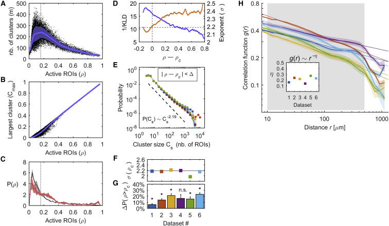
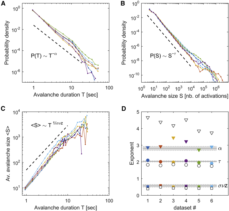
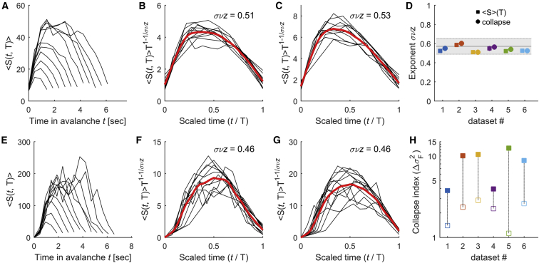
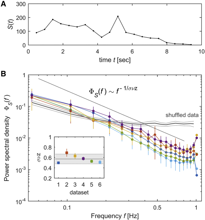
Previous studies suggest that the brain operates at a critical point in which phases of order and disorder coexist, producing emergent patterned dynamics at all scales and optimizing several brain functions. Here, we combined light-sheet microscopy with GCaMP zebrafish larvae to study whole-brain dynamics in vivo at near single-cell resolution. We show that spontaneous activity propagates in the brain's three-dimensional space, generating scale-invariant neuronal avalanches with time courses and recurrence times that exhibit statistical self-similarity at different magnitude, temporal, and frequency scales. This suggests that the nervous system operates close to a non-equilibrium phase transition, where a large repertoire of spatial, temporal, and interactive modes can be supported. Finally, we show that gap junctions contribute to the maintenance of criticality and that, during interactions with the environment (sensory inputs and self-generated behaviors), the system is transiently displaced to a more ordered regime, conceivably to limit the potential sensory representations and motor outcomes.

Keywords: GcaMP; calcium imaging; gap junctions; light-sheet microscopy; motor behavior; phase transitions; scale invariance; sensory modulation; whole-brain dynamics; zebrafish.


Figures

Figure 1
Figure 1
Statistics of the Clusters of Co-active and Contiguous ROIs (A) Number of clusters (m) as a function of the proportion of active ROIs (ρ). Blue line, mean of m; blue area, its standard deviation. (B) Normalized size of the largest cluster (Cmax) as a function of ρ (blue trace: average Cmax). (C) Distribution of ρ (black, spontaneous activity; red, stimulus-evoked activity) calculated for each of the Q spontaneous and evoked segments (solid line, mean distribution; shaded area, SEM). Note that the stimulus-evoked distribution is skewed to the right. (D) We calculated the cluster size distribution for the set of clusters that appeared with ρ comprised within small intervals (ρ – Δ; ρ + Δ). Using the Kullback-Leibler divergence (KLD), we calculated the goodness of fit of the power law (blue) and, using MLE, we estimated the power exponent (orange) as a function of ρ. (A)–(D) show results for dataset 1. Note that, for ρ = ρc, the goodness of fit is close to its maximum and the corresponding power exponent is equal to one predicted in the case of 3D percolation, equal to 2.19 (dashed horizontal line). (E) Size distribution P(Cs) of clusters that appeared with ρ between ρc – Δ and ρc + Δ. Each color represents a dataset. Error bars are smaller than the symbols’ size. Black line, power-law distribution predicted in 3D percolation. (F) Power exponents σ(ρc) estimated using MLE. (G) Difference between the proportion of time that ρ > ρc during the stimulus-evoked activity and the proportion of time that ρ > ρc during the spontaneous activity (p < 0.01, paired t test). Error bars, SEM across the Q spontaneous-evoked segments. See also Figure S2. (H) Correlation function g(r): average correlation between pairs of cells as a function of the Euclidean distance r, for each dataset (calculated for each of the Q segments and then averaged; colored areas, SEM). The straight lines represent power-law fits using least squares for r falling between 50 μm and 500 μm (gray area). Note that for distances longer than 500 μm, r approximates the size of the larva in one of its 3 dimensions. Inset: estimated power-law exponent (estimation errors are smaller than the symbols’ size).
Figure 2
Figure 2
Neuronal Avalanches Show Critical Statistics (A) Distribution of avalanche durations T (in s). (B) Distribution of avalanche sizes S (i.e., cumulative sum of the number of activated ROIs). (C) Relation between S and T, for each dataset. In (A), (B), and (C), each color corresponds to a dataset and the black dashed line indicates the power law expected in the case of critical behavior. The validity of the power-law fitting was evaluated using Kolmogorov-Smirnov statistics and log-likelihood ratio tests; see Table S2 for more details. (D) Measured exponents for each dataset (colored filled symbols) and the corresponding time-shuffled data (open symbols). Triangles, α exponent; circles, τ exponent; squares, σνz exponent. Error bars (estimation errors) are smaller than the size of the symbols. The gray horizontal lines and the gray shaded areas indicate the expected critical exponents and their uncertainty, respectively, in 3D random field Ising models. See Table S2 for more details. See also Figures S3 and S4.
Figure 3
Figure 3
Universal Scaling Functions: Avalanche Profiles (A) Averaged temporal profile, S(t,T), of avalanches of durations T, where T = 2.82 – 7.99 s (data from dataset 3). (B) Scaled avalanche profiles as a function of the scaled time t/T. Red line, averaged scaled avalanche profile; σνz, best scaling parameter (data from dataset 3). (C) Same as (B) but for dataset 6. (D) Estimated σνz exponents using scaling collapse (circles) and the relation S(T) (squares). Each color represents a different dataset. Estimation errors are smaller than the size of the symbols. Note the similarity between the exponents calculated with the two different methods. The gray area indicates the theoretically expected critical exponent and its uncertainty. See Table S2 for more details. (E–G) Same as (A)–(C), respectively, but for the corresponding time-shuffled datasets, for which collapse was substantially reduced. (H) Amount of collapse (ΔσF2) for the original datasets (filled symbols) and the shuffled datasets (open symbols).
Figure 4
Figure 4
Universal Scaling Functions: Power Spectrum of Avalanche Time Courses (A) Temporal profile S(t) of an example avalanche of duration 9.4 s. (B) We calculated the power spectral density (PSD) of the time courses of neuronal avalanches. Each color represents a different dataset. Error bars indicate SEM. The PSD of avalanche time courses, ΦS(f), decays approximately as a power law of the frequency f with an exponent equal to 1/σνz (black line). In contrast, the PSD of time-shuffled data was uniform across frequencies and largely deviated from the predicted power law (the gray solid line is the mean PSD across shuffled datasets, and the thin gray lines depict SEM). Inset: exponent σνz estimated using least-squares for each dataset. Error bars indicate the exponent estimation error. The values of σνz estimated using this analysis are close to the expected critical exponent (0.57) indicated by the solid black line; the gray shaded area indicates the uncertainty of the critical exponent.
Figure 5
Figure 5
Universal Scaling Functions: Recurrence Time Intervals (A) Recurrence time distributions P(Δt,S>s). The distributions of time intervals Δt between consecutive avalanches of sizes larger than a given threshold s were calculated for different values of s (gray color code; data from dataset 2). (B) Rescaled recurrence time distributions as a function of the rescaled time Δt/Δt. The black curve indicates the gamma distribution onto which the scaled recurrence time distributions collapsed (γ: shape parameter of the gamma distribution; data from dataset 2). (C and D) Same as (A) and (B), respectively, but for dataset 3. See Table S2 for more details. (E–G) Same as (A), (B), and (D), respectively, but for the corresponding shuffled datasets. Note the absence of collapse for the shuffled data. (H) Amount of collapse (ΔσG2) for the original datasets (filled symbols) and the shuffled datasets (open symbols).
Figure 6
Figure 6
Propagation of Neuronal Avalanches (A and B) Probability distribution of the projection of the velocity vector into the coronal (x-y) plane of the brain, Vxy, for two representative datasets (A, dataset 1; B, dataset 2). The probability density is shown in color scale. (C) Probability distribution of the direction of propagation in the coronal (x-y) plane, θ, for each dataset. (D) Left: distribution of velocity magnitude. Right: differences in median velocities ΔV of the avalanches during periods of spontaneous and the stimulus-driven activity. p < 0.001, two-sided Wilcoxon rank-sum test. (E) Left: probability distribution of the distance traveled by the neuronal avalanches. Right: differences in median distances ΔD of the avalanches during periods of spontaneous and the stimulus-driven activity (p > 0.05, two-sided Wilcoxon rank-sum test). (F) Locations of the initial centers of mass (i.e., CM(t=1)), of neuronal avalanches projected on the coronal (x-y) plane of the brain (for dataset 1). Each green dot corresponds to an avalanche. Note that the vast majority of the initiation sites occurred in the neuronal somata rather than in the neuropil (dense white regions). (G) Probability distribution of the number of simultaneous avalanches, Ns, normalized by its mean Ns, for each dataset (solid lines). The narrow distributions are the expected Poisson distributions given Ns. (H) Probability distribution of detecting two simultaneous avalanches with CMs separated by a distance d, for each dataset. Points indicate distance bins for which the probability of simultaneous avalanches is significantly (p < 0.01) higher than chance (i.e., randomized data; see STAR Methods). See also Figure S5.
Figure 7
Figure 7
Sensory Stimulation and Self-Generated Behavior Transiently Deviate the Brain’s Dynamical State from Criticality (A–D) The average rate of avalanche initiation (A), the average avalanche size (B), and the average power exponents of the distribution of avalanche sizes (C) and durations (D) were calculated for avalanches included within sliding time windows, for all spontaneous and evoked segments and all datasets. Shaded areas indicate SEM. We compared the values during periods of spontaneous activity (black horizontal line) and during periods of visual stimulation (gray horizontal line) using a two-sided Wilcoxon rank-sum test (p, p value). We also compared the values measured in all windows during spontaneous activity using a RM-ANOVA; pA indicates the resulting p value (high p values suggest that avalanche properties were constant during periods of spontaneous activity). (E and F) Averaged exponents describing the distributions of durations (E) and sizes (F) of spontaneous neuronal avalanches around self-generated tail movement onsets. Exponents were normalized by the corresponding averaged values during the reference periods (from –100 to –10 s and from +10 to +100 s, shaded areas; with respect to movement onsets, white areas). (G and H) Averaged changes of the Kullback-Leibler divergence (KLD) between the distributions of durations (G) and sizes (H) of spontaneous avalanches and theoretical power laws (relative to reference periods). In (E)–(H), p < 0.001, two-sample t test comparing values at movement onset and values in the absence of movements. See also Figures S6 and S7.
Figure 8
Figure 8
Gap Junctions Play a Role in Maintaining Criticality in the Nervous System (A) Average distribution exponents (α, τ, σνz) of spontaneous neuronal avalanches displayed by larvae in normal experimental conditions (datasets 1–6; black bars) and by larvae exposed to heptanol (90 μM) (datasets 7 and 8; white bars). For comparison, the gray bars indicate the critical exponents of 3D random field Ising theoretical models. (B and C) Profile (B) and recurrence-time (C) collapse indices of neuronal avalanches calculated in normal conditions (black bars) and under heptanol exposure (white bars). In (A)–(C), p indicates the p value of two-sample t tests; p < 0.05, ∗∗p < 0.01. Error bars, SEM. (D) Decoding of visual stimuli at one optical plane of the optic tectum (n = 14 larvae, 8 in normal conditions and 6 after expsure to heptanol at 90 μM). Stimuli consisted of single light spots randomly presented at 4 possible closely spaced azimuth locations in the visual field (75°, 85°, 90°, and 110°). A maximum likelihood decoder was used to classify the stimuli location based on the activity of n ROIs. For n > 100, the classification performance was significantly higher than chance (i.e., 25%) for larvae in normal conditions. However, the decoding efficiency was significantly lower for larvae exposed to heptanol. p < 0.001, two-sample t test. (E) Decoding confusion matrices averaged across larvae in normal conditions (left) and across larvae exposed to heptanol (right), for n = 1,000. The off-diagonal matrix elements represent the probability of erroneously classifying one stimulus as a different one. The diagonal corresponds to correct classifications. Notice that, as expected, the decoder confused nearby stimuli. See also Figure S8.

Comment in

  • Cracklin' Fish Brains.
    Beenhakker MP. Beenhakker MP. Epilepsy Curr. 2019 Mar-Apr;19(2):112-114. doi: 10.1177/1535759719835348. Epilepsy Curr. 2019. PMID: 30955431 Free PMC article.

References

    1. Ahrens M.B., Orger M.B., Robson D.N., Li J.M., Keller P.J. Whole-brain functional imaging at cellular resolution using light-sheet microscopy. Nat. Methods. 2013;10:413–420. - PubMed
    1. Alstott J., Bullmore E., Plenz D. Powerlaw: a Python package for analysis of heavy-tailed distributions. PLoS ONE. 2014;9:e85777. - PMC - PubMed
    1. Avitan L., Pujic Z., Hughes N.J., Scott E.K., Goodhill G.J. Limitations of neural map topography for decoding spatial information. J. Neurosci. 2016;36:5385–5396. - PMC - PubMed
    1. Beggs J.M., Plenz D. Neuronal avalanches in neocortical circuits. J. Neurosci. 2003;23:11167–11177. - PMC - PubMed
    1. Bellay T., Klaus A., Seshadri S., Plenz D. Irregular spiking of pyramidal neurons organizes as scale-invariant neuronal avalanches in the awake state. eLife. 2015;4:e07224. - PMC - PubMed

Publication types

LinkOut - more resources