. 2018 Dec 3;28(23):3723-3735.e6.
doi: 10.1016/j.cub.2018.10.017. Epub 2018 Nov 15.

Whole-Brain Calcium Imaging during Physiological Vestibular Stimulation in Larval Zebrafish

Affiliations

Whole-Brain Calcium Imaging during Physiological Vestibular Stimulation in Larval Zebrafish

Geoffrey Migault et al. Curr Biol. .

Abstract

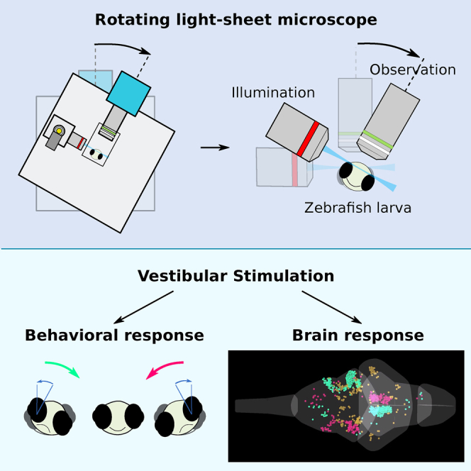
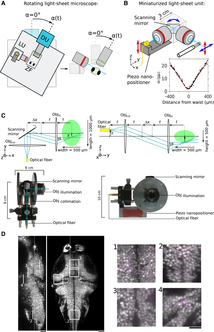
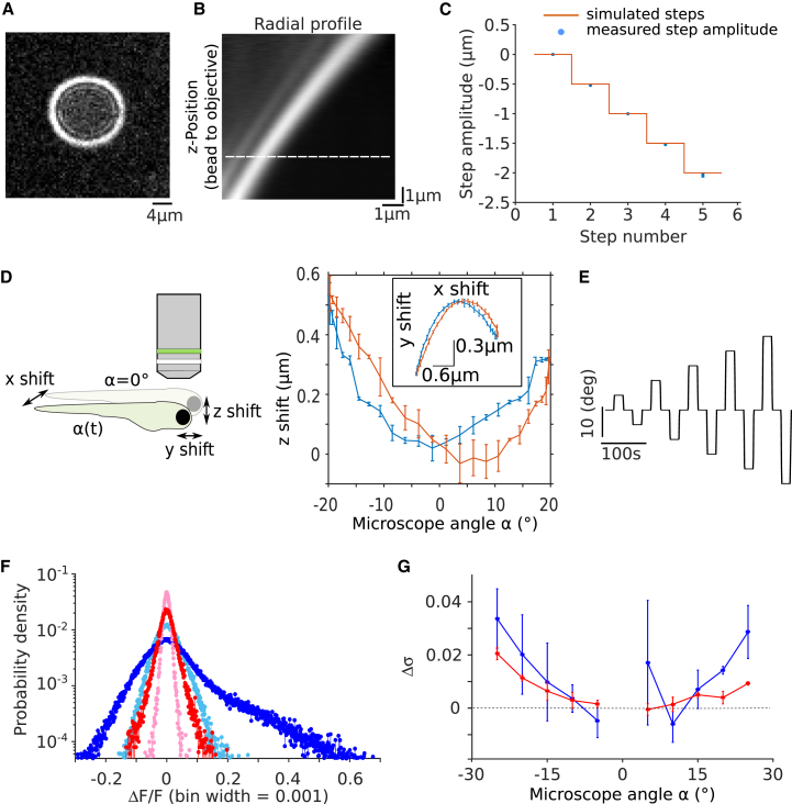
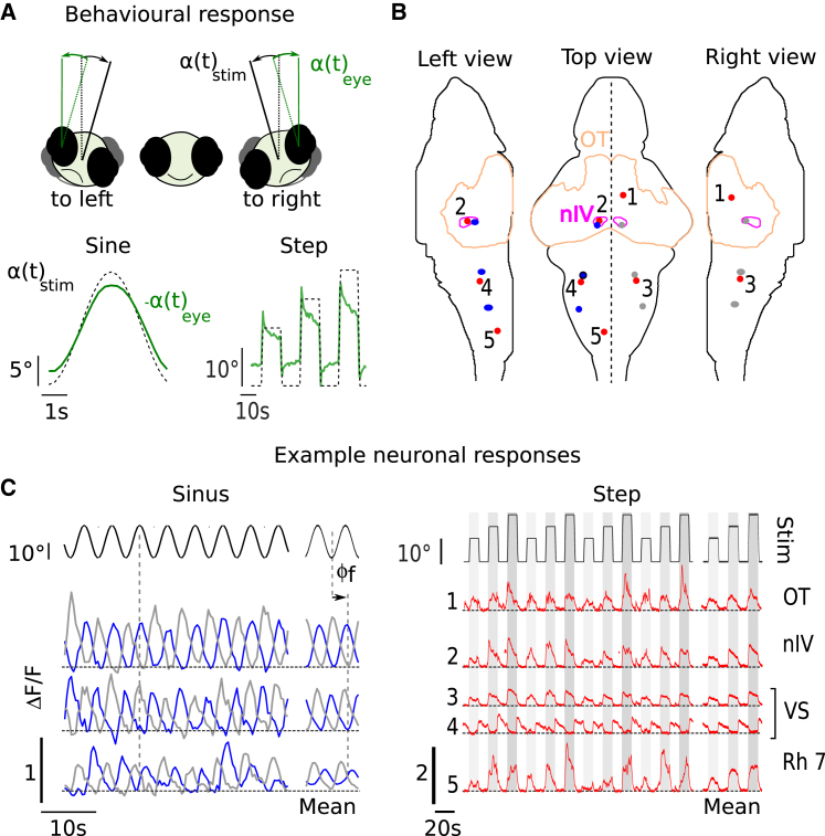
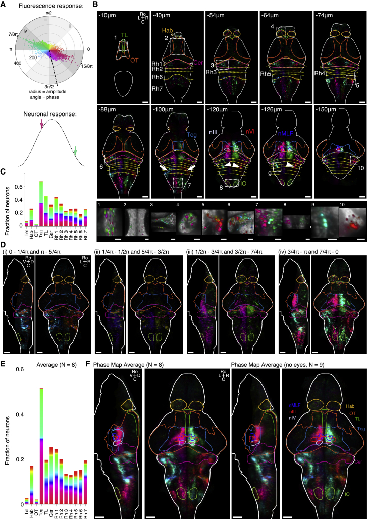
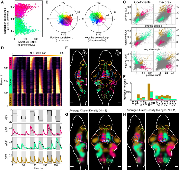
The vestibular apparatus provides animals with postural and movement-related information that is essential to adequately execute numerous sensorimotor tasks. In order to activate this sensory system in a physiological manner, one needs to macroscopically rotate or translate the animal's head, which in turn renders simultaneous neural recordings highly challenging. Here we report on a novel miniaturized, light-sheet microscope that can be dynamically co-rotated with a head-restrained zebrafish larva, enabling controlled vestibular stimulation. The mechanical rigidity of the microscope allows one to perform whole-brain functional imaging with state-of-the-art resolution and signal-to-noise ratio while imposing up to 25° in angular position and 6,000°/s2 in rotational acceleration. We illustrate the potential of this novel setup by producing the first whole-brain response maps to sinusoidal and stepwise vestibular stimulation. The responsive population spans multiple brain areas and displays bilateral symmetry, and its organization is highly stereotypic across individuals. Using Fourier and regression analysis, we identified three major functional clusters that exhibit well-defined phasic and tonic response patterns to vestibular stimulation. Our rotatable light-sheet microscope provides a unique tool for systematically studying vestibular processing in the vertebrate brain and extends the potential of virtual-reality systems to explore complex multisensory and motor integration during simulated 3D navigation.

Keywords: 4D data visualization; calcium imaging; functional whole-brain imaging; light-sheet microscopy; microscopy development; regression analysis; sensory processing; vestibular system; zebrafish.


Figures

None
Graphical abstract
Figure 1
Figure 1
Experimental Setup and Imaging Performance (A) Schematic of the rotating microscope setup with the light-sheet unit (LU), mounted zebrafish (ZF), and detection unit (DU). The close-up image illustrates how the fish rotates together with the microscope such that the light sheet and the detection focal plane coincide for any rotation angle. Stimulation angles are counted as positive in the direction indicated by the arrow. The fish faces the breadboard with its long body axis aligned with the microscope rotation axis. (B) Schematic of the light-sheet-forming unit. Inset: measured light-sheet profile (black) and adjusted with the theoretical Gaussian beam profile (red). (C) Details of the light-sheet unit. The left part illustrates in a top view the scanning mechanism for the light-sheet formation. The right part illustrates in a side view the ray diagram for the z scanning of the light sheet. The scanning mirror is omitted for clarity. The green ellipse schematizes the fluorescent zebrafish brain. The photographs of the light-sheet unit corresponding to top and side views are shown below the two schemes. The two metallic disks allow rotating the unit for alignment. (D) Sagittal and coronal sections of a volumetric whole-brain scan of a 6-day-old zebrafish larva with pan-neuronal GCaMP6s expression (Tg(elavl3:H2B-GCaMP6s)). The four insets show quasi-single-cell resolution and the result of the automatic segmentation process. Scale bars, 50 μm (main image) and 25 μm (insets). See also Video S1.
Figure 2
Figure 2
Stability Characterization and Noise-Level Estimation (A) Characteristic interference pattern of a fluorescent microsphere displaced relative to the focal plane of the detection objective. (B) Radial intensity profile averaged over all angles as a function of the imposed objective height. This profile serves as a look-up table (LUT) to quantify z movements of the microsphere during microscope rotation. The dashed line indicates the fit position for the profile shown in (A). (C) Performance test of the z tracking algorithm. A control signal drives a piezo to displace the detection objective in steps of 0.5 μm (red), and the relative distance of the microsphere to the objective (blue; error bars indicate SD; N = 5) is computed by fitting the instantaneous intensity profile of the microsphere onto the LUT shown in (B). (D) Characterization of the shift along the z direction of the scanned volume as a function of the microscope rotation angle (blue; error bars indicate SD, N = 5). Rotation direction is from −20° to +20° in blue and the reverse rotation is in red. The inset shows the corresponding movements in the x-y plane. The schematic defines the coordinate system. (E) Step stimulation protocol used for estimating the mechanically induced noise level. (F) Distribution of the intensity change per pixel induced by a −15° microscope rotation relative to the intensity value measured just before the step (RFP- [red] and GCaMP6s- [blue] expressing fish). Light colors correspond to the intrinsic noise distribution measured in the absence of microscope rotation. Data were centered and normalized via Gaussian fits. (G) Mean mechanically induced noise level (Δσ) measured with RFP- (red) and GCaMP6s- (blue) expressing fish as a function of microscope angle (error bars indicate SD; N = 3 fish).
Figure 3
Figure 3
Behavioral and Neuronal Response to Sinusoidal and Stepwise Dynamic Vestibular Stimulation (A) Top: schematic illustrating the rolling rotation of the fish when the microscope rotates and the evoked compensatory eye movements. Angles are counted as positive in the clockwise direction, i.e., when the fish rolls toward its right side. Bottom: trial-averaged behavioral response to sinusoidal and to step stimulation (dashed black) and associated compensatory eye movements (green). The sign of the eye orientation has been reversed to facilitate comparison. (B) Three views showing the location of the regions of interest (red, blue, and gray disks) in Z-Brain coordinates from which the fluorescence example time traces shown in (C) were extracted. The outline of the optic tectum (OT) and the trochlear nucleus (nIV) are shown. (C) Example fluorescence traces (raw signals and trial average). Horizontal dashed lines indicate zero, which is defined by the calculated fluorescence baseline (see STAR Methods). Left: responses to sinusoidal stimulation (blue and gray disks from rostral to caudal in B). Right: responses to step stimulation (red-numbered disks). OT, optic tectrum; nIV, trochlear nucleus; VS, vestibulo-spinal neurons; Rh, rhombomere. All data were recorded with Tg(elavl3:GCaMP6s) fish. See also Video S2.
Figure 4
Figure 4
Phase Maps of Functional Brain-wide Response to Sinusoidal Vestibular Rolling Stimulation, Paralyzed Fish (A) Top: polar plot of the fluorescence response amplitude per neuron measured in units of signal to noise (STAR Methods) and plotted against the phase delay of the response relative to the stimulus. The color code indicates the phase shift. The dashed line indicates the expected position of a zero-phase-shift neuronal signal once corrected for the phase delay introduced by the GCaMP6s sensor (STAR Methods). Bottom: schematic showing one stimulus cycle (black dashed). Arrows indicate the phase in the cycle where the neurons with the dominant response (black line, top) have their maximal response when taking into account the delay introduced by the GCaMP6s sensor. (B) Top: ten selected phase map layers of an example fish after registration on the Z-Brain reference brain. The delineated brain areas are from the Z-Brain atlas. Bottom: close-up views of regions shown by the dashed rectangles. (C) Fractions of responding neurons and the corresponding phase-shift distribution in the 13 selected brain areas. (D) Maximum-projection views of the phase map shown in (B) and separated into the four phase intervals depicted in (A). For each phase interval, a maximum projection from left to the midline and from dorsal to ventral is shown. (E) Fraction of responding neurons and the corresponding phase distribution for the 13 selected brain areas. (F) Average phase maps. Left: average of N = 8 paralyzed fish. Right: average of N = 9 bi-enucleated paralyzed fish. Maximum projections from left to the midline and from dorsal to ventral are shown. C, caudal; D, dorsal; Hab, habenula; IO, inferior olive; L, left; R, right; Ro, rostral; TL, torus longitudinalis; Teg, tegmentum; nMLF, nuclear medial fasciculus; nIII, oculomotor nucleus; nIV, trochlear nucleus; Cer, cerebellum; V, ventral; Rh, rhombomere. All data were recorded in Tg(elavl3:H2B-GCaMP6s) fish. Scale bars, 50 μm and 20 μm (close-up views in B). See also Figures S2–S4 and Videos S3 and S4.
Figure 5
Figure 5
Functional Brain-wide Neuronal Response to Dynamic Vestibular Step Stimulation, Paralyzed Fish (A) Scatterplot showing the responsiveness of neurons to a step stimulus (correlation coefficient) versus the responsiveness to a sinusoidal stimulus (response amplitude is defined as the signal-to-noise ratio measured at the stimulation frequency; STAR Methods). Points are colored according to the phase shift of the response with respect to the sinusoidal stimulation. SNR, signal-to-noise ratio. (B) Scatterplot of all neurons (same as A), with the correlation coefficient ρ as radius and the phase as angle, using the same color code as (A). The left panel shows all points with a positive ρ, whereas the right panel shows all points with a negative ρ (radius is the absolute value of ρ). Black contour lines indicate isovalues for the density distribution. (C) Multi-regression analysis reveals three neuronal response clusters. Scatterplots of the regression coefficients (left column) and corresponding T scores (right column). Data are from the example fish shown in Video S5 and (A)–(E) and represent a total of 77,648 neurons. Neurons that do not belong to the responsive clusters are shown as gray dots; clustered neurons are colored according to the corresponding cluster color. The magenta cluster corresponds to neurons that display strong response to both positive angle and positive angular velocity (>95th percentile in both regression coefficient and associated T score). Neurons of the pale green cluster are highly responsive to both negative angle and negative angular velocity, whereas neurons from the golden cluster show high response to both positive and negative angular velocity. (D) Top: trial-averaged traces of all neurons in the three clusters to stepwise stimulation. Neuron index is denoted on the left (1–1,168), ΔF/F scale color bar is shown at the top (values are clipped to [0, 0.5]), and neuron cluster assignment is shown in the color bar on the left. Neurons are grouped by cluster and subsequently sorted by coefficient strength to the position regressor, to show the gradient in response strengths. Bottom: rotation angle α of the vestibular step stimulus (black) and the trial- and neuron-averaged traces of the three clusters in their respective colors. Additionally, their mean regression fit is plotted (black filled line), and for the magenta cluster and pale green cluster the mean position-only fit is plotted (black dashed line) to illustrate the contribution of each regressor. (E) Visualization of the cluster spatial organization performed for the same example fish with the Fishualizer. These data are also shown in Video S5, part II in 3D. (F) The histogram shows for selected brain regions the fraction of neurons that are part of the three identified average cluster densities. Tel, telencephalon; Hab, habenula; PT, pretectum; DTh, dorsal thalamus; VTh, ventral thalamus; OT, optic tectum; TSC, torus semicircularis; Teg, tegmentum; TL, torus longitudinalis; Cer, cerebellum; Rh 1–7, rhombomere 1–7. (G) Visualization of the average density map of N = 8 paralyzed fish with eyes. 3D visualization is in Video S5, part III. Color intensity scales linearly with density. Outlines of the indicated brain regions from rostral to caudal: habenula, torus longitudinalis, tegmentum, optic tectum, nMLF, oculomotor nucleus nIII, trochlear motor nucleus nIV, cerebellum, and inferior olive. (H) Average density map of N = 11 bi-enucleated fish. All data were recorded in Tg(elavl3:H2B-GCaMP6s) fish. Scale bars, 50 μm. See also Figure S5 and Video S5.

Comment in

Similar articles

Cited by

References

    1. Panier T., Romano S.A., Olive R., Pietri T., Sumbre G., Candelier R., Debrégeas G. Fast functional imaging of multiple brain regions in intact zebrafish larvae using selective plane illumination microscopy. Front. Neural Circuits. 2013;7:65. - PMC - PubMed
    1. Ahrens M.B., Orger M.B., Robson D.N., Li J.M., Keller P.J. Whole-brain functional imaging at cellular resolution using light-sheet microscopy. Nat. Methods. 2013;10:413–420. - PubMed
    1. Wolf S., Supatto W., Debrégeas G., Mahou P., Kruglik S.G., Sintes J.-M., Beaurepaire E., Candelier R. Whole-brain functional imaging with two-photon light-sheet microscopy. Nat. Methods. 2015;12:379–380. - PubMed
    1. Ahrens M.B., Li J.M., Orger M.B., Robson D.N., Schier A.F., Engert F., Portugues R. Brain-wide neuronal dynamics during motor adaptation in zebrafish. Nature. 2012;485:471–477. - PMC - PubMed
    1. Keller P.J., Ahrens M.B. Visualizing whole-brain activity and development at the single-cell level using light-sheet microscopy. Neuron. 2015;85:462–483. - PubMed

Publication types

LinkOut - more resources