The environmental costs and benefits of high-yield farming

Abstract

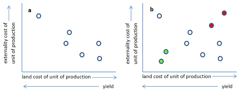
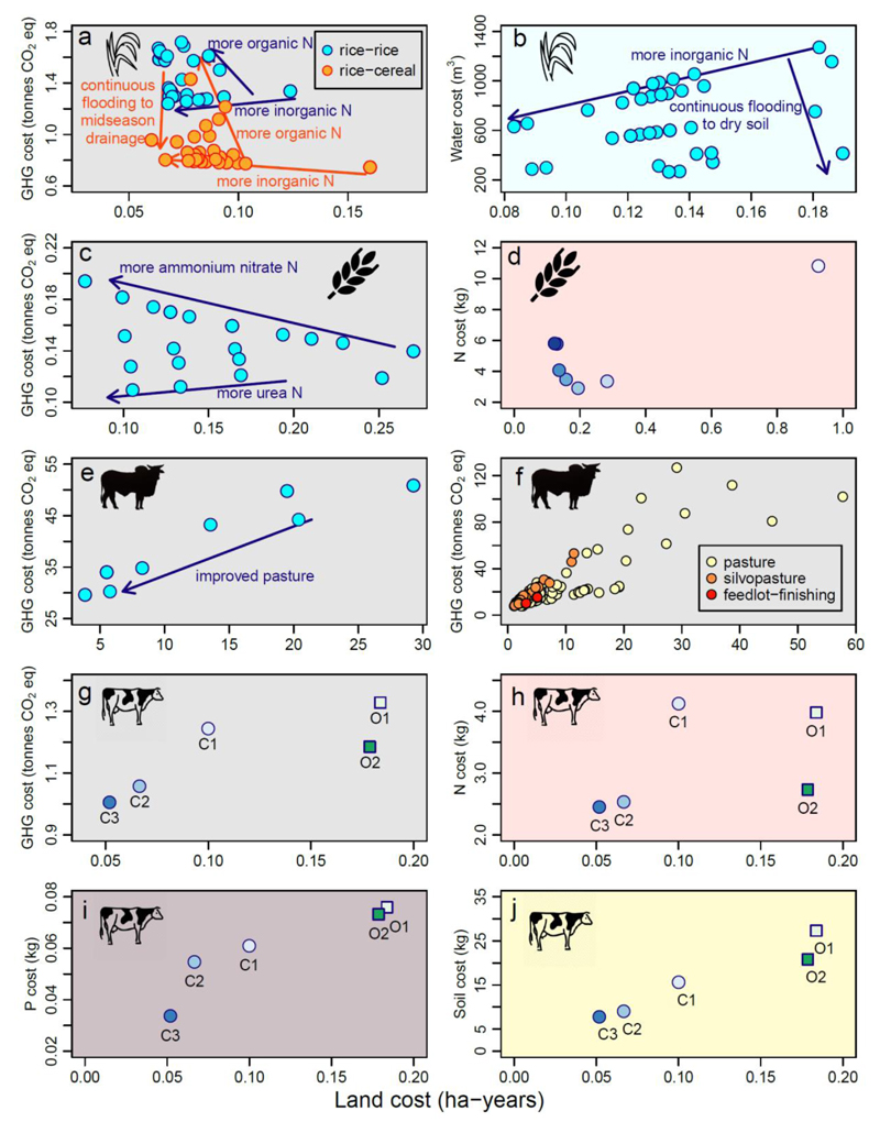
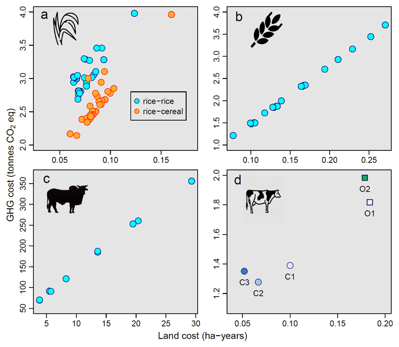
How we manage farming and food systems to meet rising demand is pivotal to the future of biodiversity. Extensive field data suggest impacts on wild populations would be greatly reduced through boosting yields on existing farmland so as to spare remaining natural habitats. High-yield farming raises other concerns because expressed per unit area it can generate high levels of externalities such as greenhouse gas (GHG) emissions and nutrient losses. However, such metrics underestimate the overall impacts of lower-yield systems, so here we develop a framework that instead compares externality and land costs per unit production. Applying this to diverse datasets describing the externalities of four major farm sectors reveals that, rather than involving trade-offs, the externality and land costs of alternative production systems can co-vary positively: per unit production, land-efficient systems often produce lower externalities. For GHG emissions these associations become more strongly positive once forgone sequestration is included. Our conclusions are limited: remarkably few studies report externalities alongside yields; many important externalities and farming systems are inadequately measured; and realising the environmental benefits of high-yield systems typically requires additional measures to limit farmland expansion. Yet our results nevertheless suggest that trade-offs among key cost metrics are not as ubiquitous as sometimes perceived.

Fig. 1. Framework for exploring how different environmental costs compare across alternative production systems.

a, Hypothetical plot of externality cost vs land cost of different, potentially interchangeable production systems (blue circles) in a given farming sector. In this example the data suggest a trade-off between externality and land costs across different systems. b, This example reveals a more complex pattern, with additional systems (in green and red circles) that are low or high in both costs.

Fig. 2. Externality costs of alternative production systems against land cost for five externalities in four agricultural sectors.

All costs are expressed per tonne of production (so land cost, for instance, is in ha-years/tonne– i.e. the inverse of yield). Different externalities are indicated by background shading (grey = GHG emissions, blue = water use, pink = N emissions, purple = P emissions, buff = soil loss), and different sectors (Asian paddy rice, European wheat, Latin American beef, European dairy) are shown by icons. Points on plots derived from multi-site experiments (a, b, c) and LCAs (e) show values for systems adjusted for site and study effects via GLMMs of land cost and externality cost (for 95% confidence intervals, see Supplementary Fig. 1), while arrows show management practices with statistically-significant effects (whose 95% confidence intervals do not overlap zero in the GLMMs; Methods). In d (wheat and N emissions), progressively darker circles depict increasing nitrate application rate (0, 48, 96, 144, 192, 240 and 288 kg N/ha-year). In f (beef and GHG emissions, estimated by RUMINANT), different colours show different system types. In g-j (dairy and four externalities), circles and squares show results for conventional and organic systems, respectively (detailed in Supplementary Table 4). Spearman's rank correlation coefficients (p-values) are a. rice-rice: -0.51 (0.002), rice-cereal: -0.36 (0.06), b. 0.19 (0.26), c. -0.34 (0.14), d. -0.21 (0.66), e. 0.95 (0.001), f. 0.83 (< 0.001), g. 0.90 (0.08), h. 0.70 (0.23), i. 1.00 (0.02) and j. 1.00 (0.02). Note that these correlation coefficients do not necessarily reflect non-linear relationships (e.g., d) accurately.

Fig. 3. Overall GHG cost against land cost of alternative systems in each sector, including the GHG opportunity costs of land under farming.

Y-axis values are the sum of GHG emissions from farming activities (plotted in Figs. 2 a, c, e, g) and the forgone sequestration potential of land maintained under farming and thus unable to revert to natural vegetation (Methods). All costs are expressed per tonne of production. Notation as in Fig. 2. Spearman's rank correlation coefficients (p-values) are a. rice-rice: 0.40 (0.017), rice-cereal: 0.80 (< 0.001), b. 0.99 (< 0.001), c. 0.98 (< 0.001) and d. 0.80 (0.13).

References

1. Poore J, Nemecek T. Reducing food’s environmental impacts through producers and consumers. Science. 2018;360:987–992. - PubMed
1. Green RE, Cornell SJ, Scharlemann JPW, Balmford A. Farming and the fate of wild nature. Science. 2005;307:550–555. - PubMed
1. Tilman D, Balzer C, Hill J, Befort BL. Global food demand and the sustainable intensification of agriculture. Proc Natl Acad Sci U S A. 2011;108:20260–20264. - PMC - PubMed
1. Hunter MC, Smith RG, Schipanski ME, Atwood LW, Mortensen DA. Agriculture in 2050: recalibrating targets for sustainable intensification. Bioscience. 2017;67:386–391.
1. Godfray HCJ, et al. Food security: the challenge of feeding 9 billion people. Science. 2010;327:812–818. - PubMed