Adaptive stimulus selection for multi-alternative psychometric functions with lapses

Abstract

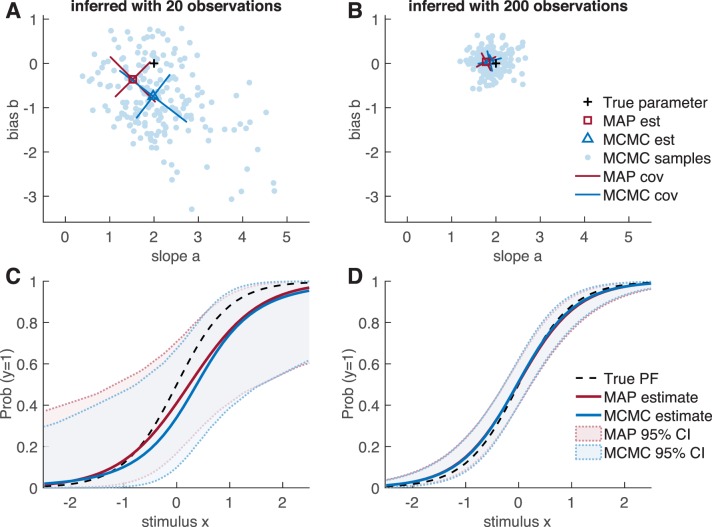
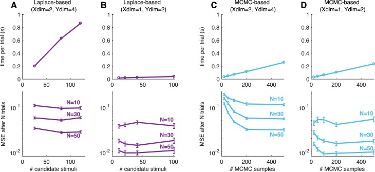
Psychometric functions (PFs) quantify how external stimuli affect behavior, and they play an important role in building models of sensory and cognitive processes. Adaptive stimulus-selection methods seek to select stimuli that are maximally informative about the PF given data observed so far in an experiment and thereby reduce the number of trials required to estimate the PF. Here we develop new adaptive stimulus-selection methods for flexible PF models in tasks with two or more alternatives. We model the PF with a multinomial logistic regression mixture model that incorporates realistic aspects of psychophysical behavior, including lapses and multiple alternatives for the response. We propose an information-theoretic criterion for stimulus selection and develop computationally efficient methods for inference and stimulus selection based on adaptive Markov-chain Monte Carlo sampling. We apply these methods to data from macaque monkeys performing a multi-alternative motion-discrimination task and show in simulated experiments that our method can achieve a substantial speed-up over random designs. These advances will reduce the amount of data needed to build accurate models of multi-alternative PFs and can be extended to high-dimensional PFs that would be infeasible to characterize with standard methods.

Figure 1

(A) Schematic of Bayesian adaptive stimulus selection. On each trial, a stimulus is presented and the response observed; the posterior over the parameters θ is updated using all data collected so far in the experiment ; and the stimulus that maximizes the expected utility (in our case, information gain) is selected for the next trial. (B) A graphical model illustrating a hierarchical psychophysical-observer model that incorporates lapses as well as the possibility of omissions. On each trial, a latent attention or lapse variable a_t is drawn from a Bernoulli distribution with parameter λ, to determine whether the observer attends to the stimulus x_t on that trial or lapses. With probability 1 − λ, the observer attends to the stimulus (a_t = 0) and the response y_t is drawn from a multinomial logistic regression model, where the probability of choosing option i is proportional to . With probability λ, the observer lapses (a_t = 1) and selects a choice from a (stimulus-independent) response distribution governed by parameter vector u. So-called omission trials, in which the observer does not select one of the valid response options, are modeled with an additional response category y_t = k.

Figure 2

Effects of omission and lapse. Here we illustrate the undesirable effects of failing to take into account omission and lapse. (A) If the psychometric function (PF) follows an ideal binomial logistic model, it can be estimated very well from data. The black dashed line shows the true PF for one of the two responses (say y = R) and the gray dashed line shows the true PF for the other (say y = L), such that the two dashed curves always add up to 1. The black dots indicate the mean probability of observing this response y = R at each stimulus point x. We drew 20 observations per stimulus point, at each of the 21 stimulus points along the one-dimensional axis. The resulting estimate for P(y = 1) is shown by the solid black line. The inference method is not important for the current purpose, but we used the maximum a posteriori estimate. (B) Now suppose that some trials fell into the implicit third choice, which is omission (red dashed line). The observed probability of y = R at each stimulus point (open black circles) follows the true PF (black dashed line). But if the omitted trials are systematically excluded from analysis, as in common practice, the estimated PF (solid black line) reflects a biased set of observations (filled black circles) and fails to recover the true PF. (C) When there is a finite lapse rate (we used a total lapse of λ = 0.2, uniformly distributed to the two outcomes), the true PF (dashed black line) asymptotes to a finite offset from 0 or 1. If the resulting observations (black dots) are fitted to a plain binomial model without lapse, the slope of the estimated PF (solid black line) is systematically biased.

Figure 3

Inferring the psychometric function. Example of a psychometric problem, with a lapse-free binomial logistic model . Given a 1-D stimulus, a response was drawn from a “true” model P(y = 1) = f(b + ax) with two parameters, slope a = 2 and bias b = 0. (A–B) On the parameter space, the posterior distributions become sharper (and closer to the true parameter values) as the data-set size N increases. (A) N = 20 (small); (b) N = 200 (large). For the maximum a posteriori estimate, the mode of the distribution is marked with a square and the two standard deviations (“widths”) of its Gaussian approximation with bars. For the Markov-chain Monte Carlo sampling method, all M = 500 samples of the chain are shown with dots, the sample mean with a triangle, and the widths with bars. The widths are the standard deviations along the principal directions of the sampled posterior (eigenvectors of the covariance matrix; not necessary aligned with the a–b axes). (C–D) The accuracy of the estimated psychometric function improves with the number of observations N, using either of the two posterior inference methods (MAP or MCMC). (C) N = 20 (small); (D) N = 200 (large). The two methods are highly consistent in this simple case, especially when N is large enough.

Figure 4

Example of infomax adaptive stimulus selection, simulated with a three-alternative lapse-free model on 1-D stimuli. The figure shows how, given a small set of data (the stimulus–response pairs shown in the top row), the psychometric functions are estimated based on the accumulated data (middle row) and the next stimulus is chosen to maximize the expected information gain (bottom row). Each column shows the instance after the N observations in a single adaptive stimulus-selection sequence, for N = 10, 11, 15, and 20, respectively. In the middle row, the estimated psychometric functions (solid lines) quickly approach the true functions (dashed lines) through the adaptive and optimal selection of stimuli. This example was generated using the Laplace approximation–based algorithm, with an independent Gaussian prior over the weights with mean zero and standard deviation σ = 10.

Figure 5

The simulated experiment. (A) At each trial, a stimulus was selected from a 2-D stimulus plane with a 21 × 21 grid. The two lines, running along x₁ and x₂ respectively, indicate the cross-sections used in (C–D). Colors indicate the most likely response in the respective stimulus regime, according to the true psychometric function shown in (B), with a consistent color code. (B) Given each stimulus, a simulated response was drawn from a true model with four alternatives. Shown here is the model with lapse, characterized by a nondeterministic choice (i.e., the choice probability does not approach 0 or 1) even at an easy stimulus, far from the choice boundaries. (C–D) Examples of Laplace approximation–based inference results after 50 trials, where stimuli were selected either (C) using our adaptive infomax method or (D) uniformly, as shown at left. In both cases, the true model was lapse free, and the algorithm assumed that lapse was fixed at zero. The two sets of curves show the cross-sections of the true (dotted) and estimated (solid) psychometric functions, along the two lines marked in (A), after sampling these stimuli. (E–F) Traces of posterior entropy from simulated experiments, averaged over 100 runs each. The true model for simulation was either (E) lapse free or (F) with a finite lapse rate of λ = 0.2, with a uniform lapse scenario c_i = 1/4 for each outcome i = 1, 2, 3, 4. In algorithms considering lapse (panels on the right), the shift in posterior entropy is due to the use of partial covariance (with respect to weight) in the case of Laplace approximation. The algorithm either used the classical multinomial logistic model that assumes zero lapse (left column) or our extended model that considers lapse (right column). Average performances of adaptive and uniform stimulus-selection algorithms are plotted in solid and dashed lines, respectively; algorithms based on Laplace approximation and Markov-chain Monte Carlo sampling are plotted in purple and cyan. The lighter lines show standard-error intervals over 100 runs, which are very narrow. All sampling-based algorithms used the semiadaptive Markov-chain Monte Carlo method with chain length M = 1,000.

Figure 6

The simulated experiment, continued; results from the same set of simulated experiments as in Figure 5. (A–B) Traces of the mean squared error, where the true model was either (A) lapse free or (B) with a total lapse rate of λ = 0.2, uniformly distributed to each outcome. Standard-error intervals are plotted in lighter lines as in Figure 5E and 5F. (C) Effect of lapse, tested by adding varying total lapse rates λ. Shown are the mean squared error after N = 100 trials of each stimulus-selection algorithm, equivalent to the endpoints in (B). Error bars indicate the standard error over 100 runs, equivalent to the lighter line intervals in Figure 5E and 5F.

Figure 7

Computation time and accuracy. (A–B) The computation times for the Laplace-based algorithms grow linearly with the number of candidate stimulus points, as shown on the top panels, because one needs to perform a numerical integration to compute the expected utility of each stimulus. In general, there is a trade-off between cost (computation time) and accuracy (inversely related to the estimation error). The bottom panels show the mean squared error of the estimated psychometric function, calculated after completing a sequence of N trials, where the 10 initial trials were selected at regular intervals and the following trials were selected under our adaptive algorithm. Error estimates were averaged over 100 independent sequences. Error bars indicate the standard errors. The true model used was the same as in either (A) Figure 5, with two-dimensional stimuli and four-alternative responses, described by nine parameters; or (B) Figure 3, with one-dimensional stimuli and binary responses, with only two parameters (slope and threshold). The different rates at which the computation time increases under the two models reflect the different complexities of numerical quadrature involved. We used lapse-free algorithms in all cases in this example. (C–D) We similarly tested the algorithms based on Markov-chain Monte Carlo sampling using the two models as in (A–B). In this case, the computation times (top panels) grow linearly with the number of samples in each chain and are not sensitive to the dimensionality of the parameter space. On the other hand, the estimation-error plots (bottom panels) suggest that a high-dimensional model requires more samples for accurate inference.

Figure 8

Optimal reordering of a real monkey data set. (A) The psychometric task consisted of a 2-D stimulus presented as moving dots, characterized by a coherence and a mean direction of movement, and a four-alternative response. The four choices are color-coded consistently in (A–C). (B) The axes-only stimulus space of the original data set, with 15 fixed stimuli along each axis. Colors indicate the most likely response in the respective stimulus regime according to the best estimate of the psychometric function. (C) The best estimate of the psychometric function of monkeys in this task, inferred from all observations in the data set. (D) Stimulus selection in the first N = 100 trials during the reordering experiment, under the inference method that ignores lapse. Shown are histograms of x₂ along one of the axes, x₁ = 0, averaged over 100 independent runs in each case. (E–F) Error traces under different algorithms, averaged over 100 runs. Algorithms based on both Laplace approximation (purple) and Markov-chain Monte Carlo sampling (cyan; M = 1,000) achieve significant speedups over uniform sampling. Because the monkeys were almost lapse free in this task, inference methods that (E) ignore and (F) consider lapse performed similarly. Standard-error intervals over 100 runs are shown in lighter lines, but are very narrow.

Figure 9

Design of multidimensional stimulus space. (A–C) Three different stimulus-space designs were used in a simulated psychometric experiment. Responses were simulated according to fixed lapse-free psychometric functions (PFs), matched to our best estimate of the monkey PF (Figure 8C). Stimuli were selected within the respective stimulus spaces: (A) the cardinal-axes design, as in the original experiment; (B) the full stimulus plane, with the PF aligned to the cardinal axes of the original stimulus space; and (C) the full stimulus plane, with rotated PF. The black dots in (A–C) indicate which stimuli were sampled by the Laplace-based infomax algorithm during the first N = 100 trials of simulation, where the dot size is proportional to the number of trials in which the stimulus was selected (averaged over 20 independent runs, and excluding the 10 fixed initial stimuli). (D) The corresponding error traces, under infomax (solid lines) or uniform (dashed lines) stimulus selection, averaged over 100 runs respectively. Colors indicate the three stimulus-space designs, as shown in (A–C). Standard-error intervals over 100 runs are shown in lighter lines.

Figure 10

Statistics of the semiadaptive Markov-chain Monte Carlo algorithm in a simulated experiment, with M = 1,000 samples per chain. We used the same binomial model as in Figure 3, and the uniform stimulus-selection algorithm. (A–B) Lapse-free model. (A) The standard deviation of the samples, along each dimension of the parameter space, decreases as the learning progresses, as expected because the posterior distribution should narrow down as more observations are collected. Also shown is the scatterplot of all 1,000 samples at the last trial N = 50, where the true parameter values are (a, b) = (5, 0). (B) The mixing time of the chain (number of steps before the autocorrelation falls to 1/e) quickly converges to some small value, meaning that the sampler is quickly optimized. Autocorrelation function at the last trial N = 50 is shown. (C–D) Same information as (A–B), but with a lapse rate of λ = 0.1, with uniform lapse ().

References

1. Akrami A, Kopec C. D, Diamond M. E, Brody C. D. Posterior parietal cortex represents sensory history and mediates its effects on behaviour. Nature. (2018 Feb 15);554(7692):368–372. doi: 10.1038/nature25510. - DOI - PubMed
1. Bak J. H, Choi J. Y, Akrami A, Witten I. B, Pillow J. W. Adaptive optimal training of animal behavior. In: Lee D. D, Sugiyama M, Luxburg U. V, Guyon I, Garnett R, editors. Advances in neural information processing systems 29. Red Hook, NY: Curran Associates, Inc; (2016). pp. 1947–1955. (Eds.)
1. Barthelmé S, Mamassian P. A flexible Bayesian method for adaptive measurement in psychophysics. arXiv:0809.0387. (2008). pp. 1–28.
1. Bishop C. M. Pattern recognition and machine learning. New York: Springer; (2006).
1. Busse L, Ayaz A, Dhruv N. T, Katzner S, Saleem A. B, Scholvinck M. L, Carandini M. The detection of visual contrast in the behaving mouse. The Journal of Neuroscience. (2011);31(31):11351–11361. doi: 10.1523/JNEUROSCI.6689-10.2011. - DOI - PMC - PubMed
Publication types