Quantifying the relative importance of experimental data points in parameter estimation

Abstract

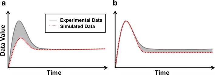
Background: Ordinary differential equations (ODEs) are often used to understand biological processes. Since ODE-based models usually contain many unknown parameters, parameter estimation is an important step toward deeper understanding of the process. Parameter estimation is often formulated as a least squares optimization problem, where all experimental data points are considered as equally important. However, this equal-weight formulation ignores the possibility of existence of relative importance among different data points, and may lead to misleading parameter estimation results. Therefore, we propose to introduce weights to account for the relative importance of different data points when formulating the least squares optimization problem. Each weight is defined by the uncertainty of one data point given the other data points. If one data point can be accurately inferred given the other data, the uncertainty of this data point is low and the importance of this data point is low. Whereas, if inferring one data point from the other data is almost impossible, it contains a huge uncertainty and carries more information for estimating parameters.

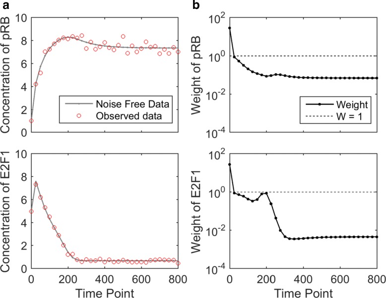
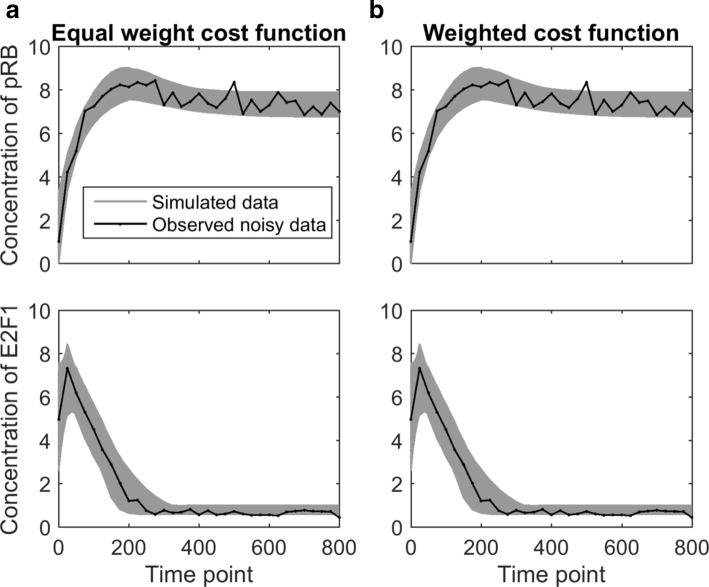
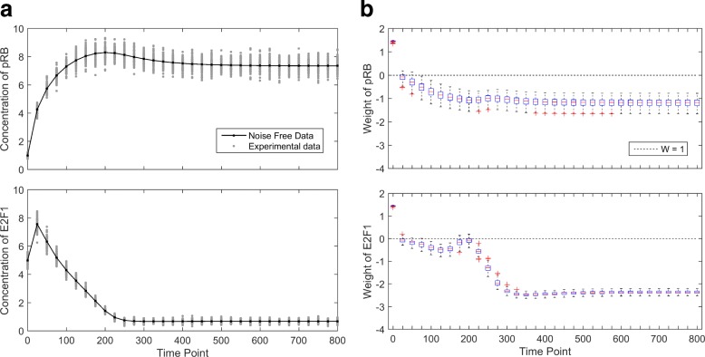
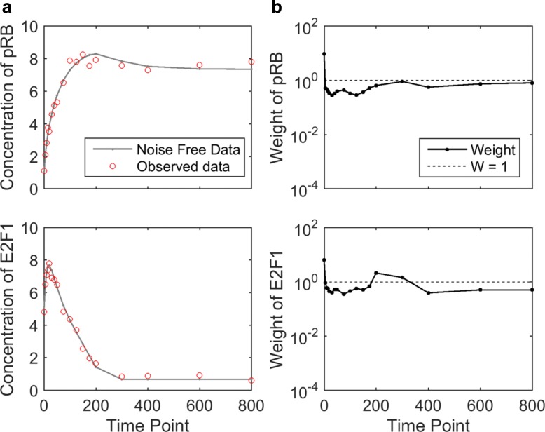
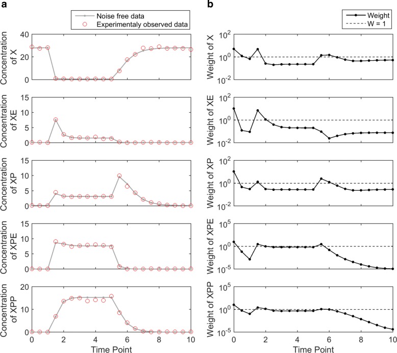
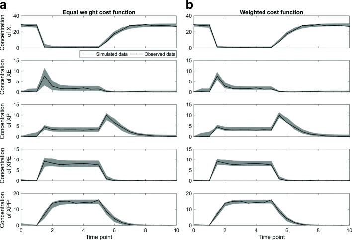
Results: G1/S transition model with 6 parameters and 12 parameters, and MAPK module with 14 parameters were used to test the weighted formulation. In each case, evenly spaced experimental data points were used. Weights calculated in these models showed similar patterns: high weights for data points in dynamic regions and low weights for data points in flat regions. We developed a sampling algorithm to evaluate the weighted formulation, and demonstrated that the weighted formulation reduced the redundancy in the data. For G1/S transition model with 12 parameters, we examined unevenly spaced experimental data points, strategically sampled to have more measurement points where the weights were relatively high, and fewer measurement points where the weights were relatively low. This analysis showed that the proposed weights can be used for designing measurement time points.

Conclusions: Giving a different weight to each data point according to its relative importance compared to other data points is an effective method for improving robustness of parameter estimation by reducing the redundancy in the experimental data.

Keywords: Ordinary differential equation; Parameter estimation; Weighted least squares.

Fig. 1

Illustrative example showing limitations of the equal-weight cost function. The solid curve represents the experimental data, and the dotted curve represents model prediction based on a parameter estimate. a A poor fit that does not capture the dynamic behavior but fits well to the flat region. b A better fit that captures the dynamic region well but is slightly off in the flat region. The shaded area represents the value of the cost function if all data points are considered as equally important. Depending on the length of the flat region, the two shaded areas (costs) can be equivalent. Therefore, the equal-weight cost function is not able to distinguish these two parameter estimates

Fig. 2

Iterative algorithm to compute uncertainty-based weights. The first iteration: parameter estimation is performed based on the equal-weight cost function using 100 random initial parameter settings obtained by Latin hypercube sampling. We pick the one with the smallest cost to calculate weights. The second and subsequent iterations: the algorithm starts with the optimized parameter from the previous iteration, and performs parameter estimation with respect to the weighted cost function using the weights from the previous iteration. The process iterates until the weights converge

Fig. 3

Experimental data and weights of the G1/S transition model with 6-parameters. a The solid curve represents the simulated noise-free data obtained from the true parameter. The circles represent simulated experimental data, which is obtained by introducing a small amount of Gaussian noise. This noisy data is used as the observed experimental data in parameter estimation. b Each dot represents the weight of a data point, and the dashed line corresponds to the weights in the equal-weight cost function (“1”). All curves are shown in log scale. The dynamic region receives relatively larger weights and the flat region receives relatively smaller weights

Fig. 4

Sampling algorithm for evaluating G1/S transition with 6-parameters. The black curve indicates the observed experimental data. The gray curves represent the model predictions based on the acceptable parameter settings, collectively forming a gray belt. a Sampling results with respect to the equal-weight cost function. The E2F1 belt from the equal-weight cost function shows imbalance between the thick width in the dynamic region and the thin width in the flat region. b Sampling results obtained from the weighted cost function. The belt width of E2F1 is much thinner in the dynamic region because the weighted cost function gives higher weights to the data points in the dynamic region. At the early time points where pRB exhibits bigger change, the pRB belt for the weighted cost function is thinner than that for the equal-weight cost function

Fig. 5

G1/S transition with 6-parameters: robustness of the uncertainty-based weights. a The black curve represents the noise-free data and the gray dots represent 100 simulated noisy datasets for sensitivity analysis. b The dotted line represents the weight of equal-weight cost function (“0” on log scale), and each box represents the weights for one data point, computed from the 100 noisy experimental datasets. The small range of each box indicates the robustness of the uncertainty-based weights

Fig. 6

Expreimental data and weights of the G1/S transition model with unevenly spaced time points. a The measurement time points are selected strategically based on the weights of the evenly spaced case. The gray dot and solid line represent the simulated noise-free data obtained from the true parameter, and the circles represent the noisy experimental data. b The black dots and solid curve represent the weights of the data points, and the dashed line represents the equal-weight cost function. The weights are very close to the dashed line except the first time point, meaning that the chosen time points are roughly equally important based on their uncertainty quantifications

Fig. 7

Experimental data and weights of the MAPK module. a The solid curve represents noise-free data obtained from the true parameter. The circles represent the noisy experimental data, generated by adding and multiplying a small amount of Gaussian noise. b Each dot represents the weight of a data point, and the dashed line corresponds to the equal-weight cost function. Data points in dynamically changing regions receive larger weights and the data points in flat regions receive relatively smaller weights

Fig. 8

Sampling algorithm for evaluating the MAPK module. The black curves show the noisy experimental data. The gray belts show the model predictions based on the acceptable parameters obtained by the sampling algorithm. By comparing the belt width of the second variable XE between the two cost functions, we can see the benefit of the weighted cost function. a The equal-weight cost function generates imbalanced belt width between dynamic regions and flat regions. b The weighted cost function produces a thin belt, meaning that it is able to better constrain the model parameters to reproduce the experimental data

Fig. 9

MAPK module: robustness of the uncertainty-based weights. a The black curve represents the noise-free data, and the gray dots represent 100 simulated noisy datasets for sensitivity analysis. b The dotted line indicates the equal-weight cost function. Each box shows the variation in of one weight caused by variations among the 100 noisy experimental datasets. Although some outliers exist, most weights exhibit small variations in this sensitivity analysis, showing the robustness of the uncertainty-based weights

References

1. Lander Arthur D. A Calculus of Purpose. PLoS Biology. 2004;2(6):e164. doi: 10.1371/journal.pbio.0020164. - DOI - PMC - PubMed
1. Sobie EA, Lee Y-S, Jenkins SL, Iyengar R. Systems biology—biomedical modeling. Sci Signal. 2011;4(190):2. doi: 10.1126/scisignal.2001989. - DOI - PMC - PubMed
1. Bartocci E, Lió P. Computational modeling, formal analysis, and tools for systems biology. PLoS Comput Biol. 2016;12(1):1–22. doi: 10.1371/journal.pcbi.1004591. - DOI - PMC - PubMed
1. Aldridge BB, Burke JM, Lauffenburger DA, Sorger PK. Physicochemical modelling of cell signalling pathways. Nat Cell Biol. 2006;8:1195–203. doi: 10.1038/ncb1497. - DOI - PubMed
1. Machado D, Costa RS, Rocha M, Ferreira EC, Tidor B, I R. Modeling formalisms in systems biology. AMB Express. 2011;1:45. doi: 10.1186/2191-0855-1-45. - DOI - PMC - PubMed
Publication types
LinkOut - more resources