Learning-based CBCT correction using alternating random forest based on auto-context model

Abstract

Purpose: Quantitative Cone Beam CT (CBCT) imaging is increasing in demand for precise image-guided radiotherapy because it provides a foundation for advanced image-guided techniques, including accurate treatment setup, online tumor delineation, and patient dose calculation. However, CBCT is currently limited only to patient setup in the clinic because of the severe issues in its image quality. In this study, we develop a learning-based approach to improve CBCT's image quality for extended clinical applications.

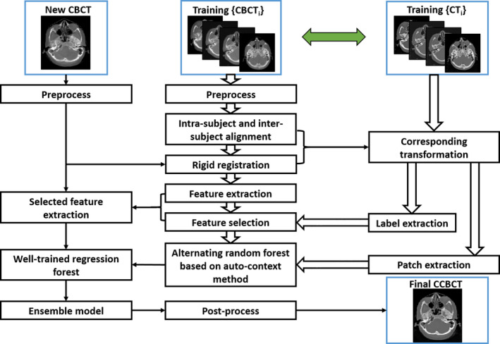
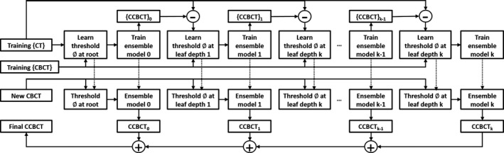
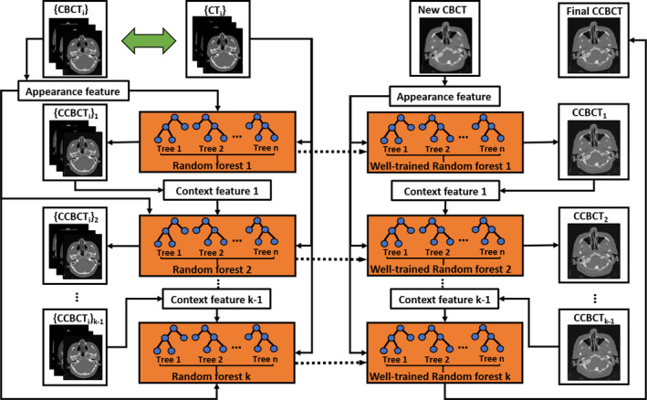
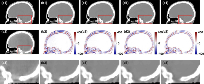
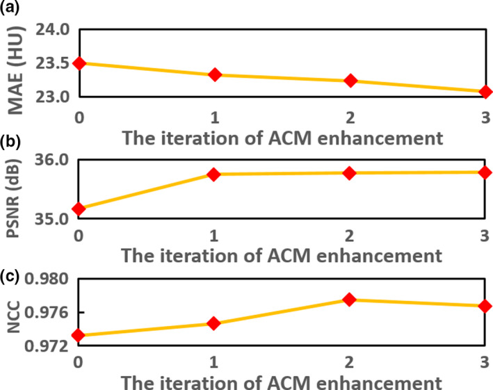
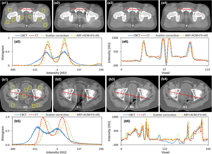
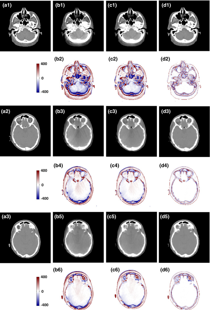
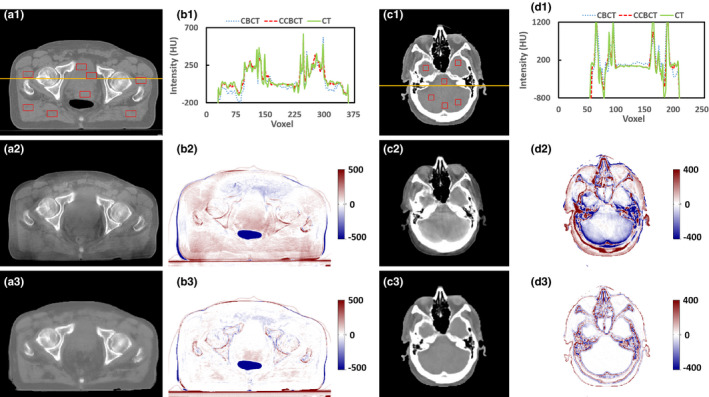
Materials and methods: An auto-context model is integrated into a machine learning framework to iteratively generate corrected CBCT (CCBCT) with high-image quality. The first step is data preprocessing for the built training dataset, in which uninformative image regions are removed, noise is reduced, and CT and CBCT images are aligned. After a CBCT image is divided into a set of patches, the most informative and salient anatomical features are extracted to train random forests. Within each patch, alternating RF is applied to create a CCBCT patch as the output. Moreover, an iterative refinement strategy is exercised to enhance the image quality of CCBCT. Then, all the CCBCT patches are integrated to reconstruct final CCBCT images.

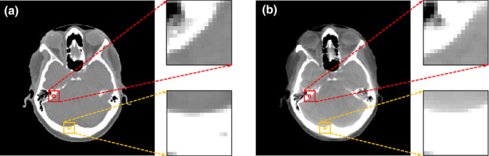
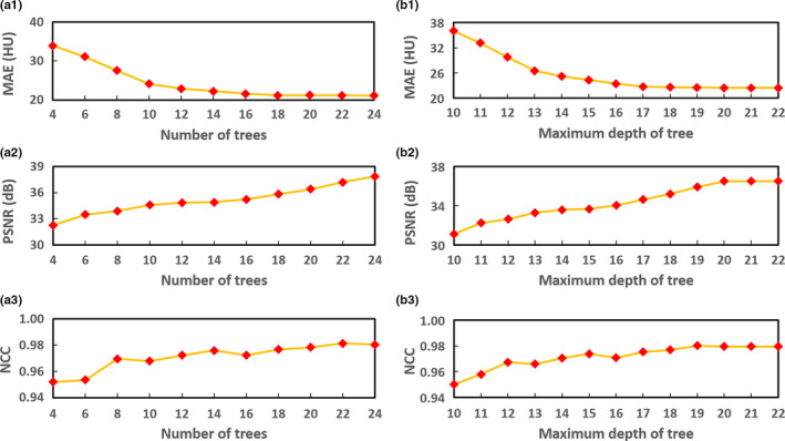
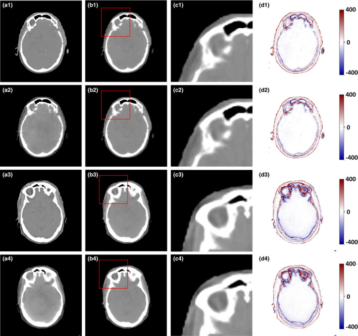
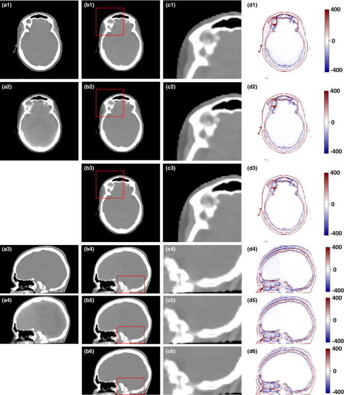
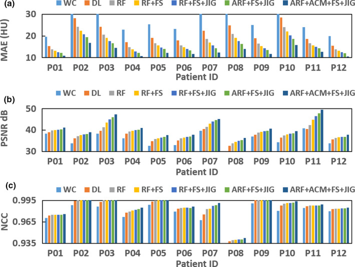
Results: The learning-based CBCT correction algorithm was evaluated using the leave-one-out cross-validation method applied on a cohort of 12 patients' brain data and 14 patients' pelvis data. The mean absolute error (MAE), peak signal-to-noise ratio (PSNR), normalized cross-correlation (NCC) indexes, and spatial nonuniformity (SNU) in the selected regions of interest (ROIs) were used to quantify the proposed algorithm's correction accuracy and generat the following results: mean MAE = 12.81 ± 2.04 and 19.94 ± 5.44 HU, mean PSNR = 40.22 ± 3.70 and 31.31 ± 2.85 dB, mean NCC = 0.98 ± 0.02 and 0.95 ± 0.01, and SNU = 2.07 ± 3.36% and 2.07 ± 3.36% for brain and pelvis data.

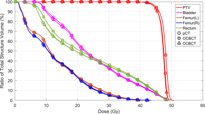
Conclusion: Preliminary results demonstrated that the novel learning-based correction method can significantly improve CBCT image quality. Hence, the proposed algorithm is of great potential in improving CBCT's image quality to support its clinical utility in CBCT-guided adaptive radiotherapy.

Keywords: CBCT correction; adaptive radiotherapy; alternating random forest; feature selection.

Figure 1

The schematic flow diagram of the proposed method. [Color figure can be viewed at wileyonlinelibrary.com]

Figure 2

An example illustrates the benefit of feature selection in material separation. [Color figure can be viewed at wileyonlinelibrary.com]

Figure 3

An example of a CT‐CBCT pair. (a) is the CT image and (b) is the corresponding CBCT image. [Color figure can be viewed at wileyonlinelibrary.com]

Figure 4

Algorithmic architecture of the alternating regression forest approach.

Figure 5

Algorithmic architecture of auto‐context modeling. [Color figure can be viewed at wileyonlinelibrary.com]

Figure 6

(a1–a3) show the performance of the proposed CBCT correction method assessed by mean absolute error (MAE), peak signal‐to‐noise ratio (PSNR) and normalized cross‐correlation (NCC), as function of the number of decision trees. (b1–b3) show the performance of the proposed CBCT correction method assessed by (a) MAE, (b) PSNR, and (c) NCC, as function of the maximum depth in decision tree. [Color figure can be viewed at wileyonlinelibrary.com]

Figure 7

Comparison of the results with and without feature selection. (a1) and (a3) are the planning CT, (a2) and (a4) are the corresponding CBCT images, (b1–d1) and (b3–d3) are the CCBCT images, zoomed regions indicated by red boxes, and difference images between planning CT and CCBCT given by RF; (b2–d2) and (b4–d4) are CCBCT images, zoomed regions indicated by red boxes, difference images between planning CT and CCBCT given by RF + FS. Display windows are [−400, 400] HU for all the subfigures. [Color figure can be viewed at wileyonlinelibrary.com]

Figure 8

Comparison of the results with different methods. (a1) and (a3) are the planning CT, (a2) and (a4) are the original CBCT images, (b1–d1) and (b4–d4) are the CCBCT images, zoomed regions indicated by red boxes, and difference images between planning CT and CCBCT given by RF + FS; (b2–d2) and (b5–d5) are the CCBCT image, zoomed regions indicated by red boxes, and difference images between planning CT and CCBCT given by RF + FS + JIG; (b3–d3) and (b6–d6) are the CCBCT image, zoomed regions indicated by red boxes, and difference images between planning CT and CCBCT given by ARF + FS + JIG. Display windows are [−400, 400] HU for all the subfigures. [Color figure can be viewed at wileyonlinelibrary.com]

Figure 9

Improvement in the performance over iterations. (a1) planning CT, (a2) CBCT, (b1–e1) CCBCT results corresponding to 1, 2, and 3 iteration of; (a2–e2) corresponding difference images between planning CT and CCBCT (b1–e1). (a3) shows the zoomed regions indicated by red boxes in (a2). (b3–e3) show the zoomed regions indicated by red boxes in (b1–e1). Display windows are [−400, 400] HU for all the subfigures. [Color figure can be viewed at wileyonlinelibrary.com]

Figure 10

(a) Improvement in the performance as assessed by (a) mean absolute error, (b) PSNR, and (c) normalized cross‐correlation, over iteration of refinement. [Color figure can be viewed at wileyonlinelibrary.com]

Figure 11

Comparison of the proposed algorithm and a conventional correction method with pelvic patient and phantom data. (a1–a6) are the phantom CT, CBCT image without correction, the result obtained by a conventional correction method, the result generated by our ARF + ACM + FS + JIG, the histogram plots in (a1–a4) and the profiles through the red solid line in (a1–a4), respectively. (b1–b6) are the patient planning CT, CBCT image without correction, the result obtained by this conventional correction method, the result generated by our ARF + ACM + FS + JIG, the histogram plots in (b1–b4) and the profiles through the red solid line in (b1–b4), respectively. Display windows are [−400, 400] HU for (a1–a4) and (b1–b4). [Color figure can be viewed at wileyonlinelibrary.com]

Figure 12

Comparison of the results with the DL‐based method, (a1–a3) are planning CT, (b1), (b3), and (b5) are the CBCT images without correction, (b2), (b4), and (b6) are the difference images between the planning CT and the CBCT without correction; (c1), (c3), and (c5) are the CCBCT results of the DL‐based method, (c2), (c4), and (c6) are the difference images between the CT and the CCBCT results achieved by DL‐based method, (d1) (d3) and (d5) are the CCBCT results of ARF + ACM + FS + JIG, (d2), (d4), and (d6) are the difference images between the planning CT and the CCBCT results obtained by ARF + ACM + FS + JIG. Display windows are [−400, 400] HU for all the subfigures. [Color figure can be viewed at wileyonlinelibrary.com]

Figure 13

(a–c) show the mean absolute error, peak signal‐to‐noise ratio, normalized cross‐correlation of different methods for each patient's brain data. [Color figure can be viewed at wileyonlinelibrary.com]

Figure 14

Evaluation of proposed algorithm with pelvic and cranial data, (a1) and (c1) are the planning CT, (a2) and (c2) are the CBCT images without correction, (b2) and (d2) are the difference images between the planning CT and the CBCT without correction; (a3) and (c3) are the CCBCT results of our ARF + ACM + FS + JIG, (b3) and (d3) are the difference images between the planning CT and the CCBCT results obtained by our ARF + ACM + FS + JIG. (b1) and (d1) are the histogram plot of orange solid line in (a1) and (c1). Display windows are [−500, 500] HU for (a1–a3) and (b2–b3), and [−400, 400] HU for (c1–c3) and (d2–d3). [Color figure can be viewed at wileyonlinelibrary.com]

Figure 15

The DVH curves of PTVs and related OARs for pelvic case. OARs for pelvis are bladder, rectum, left femur [Femur(L)], and right femur [Femur(R)]. [Color figure can be viewed at wileyonlinelibrary.com]

References

-
- Xing L, Thorndyke B, Schreibmann E, et al. Overview of image‐guided radiation therapy. Med Dosim. 2006;31:91–112. - PubMed
- Niu TY, Zhu L. Overview of x‐ray scatter in cone‐beam computed tomography and its correction methods. Curr Med Imaging Rev. 2010;6:82–89.
- Siewerdsen JH, Daly MJ, Bakhtiar B, et al. A simple, direct method for x‐ray scatter estimation and correction in digital radiography and cone‐beam CT. Med Phys. 2006;33:187–197. - PubMed
MeSH terms
Grants and funding
LinkOut - more resources
Full Text Sources
Miscellaneous