Review
. 2018 Nov 13:12:90.
doi: 10.3389/fncom.2018.00090. eCollection 2018.

The Anatomy of Inference: Generative Models and Brain Structure

Affiliations
Review

The Anatomy of Inference: Generative Models and Brain Structure

Thomas Parr et al. Front Comput Neurosci. .

Abstract

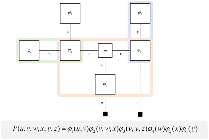
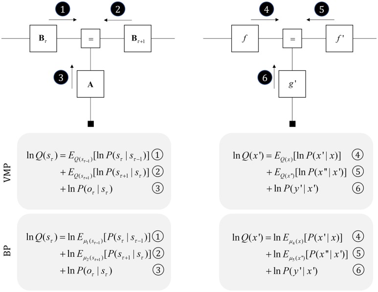
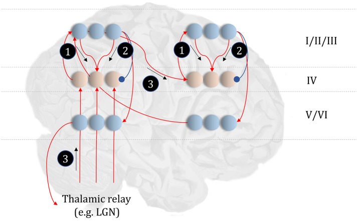
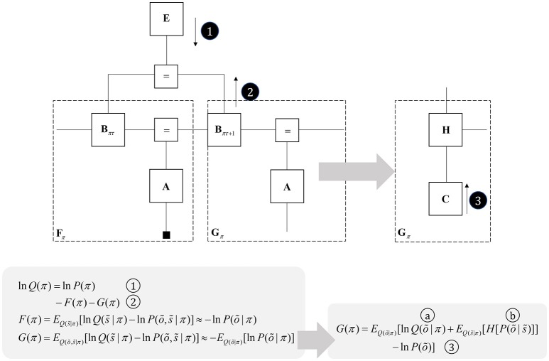
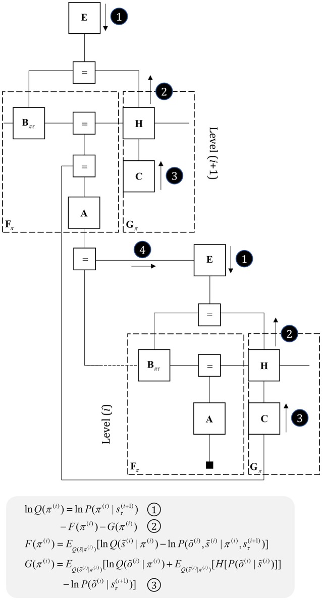
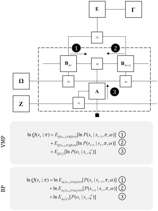
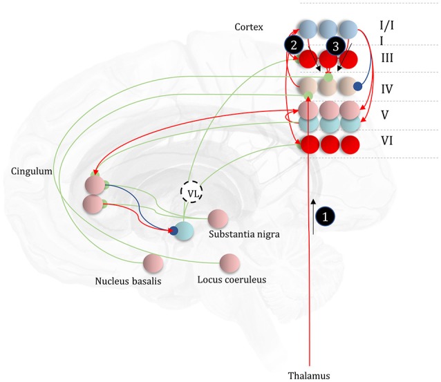
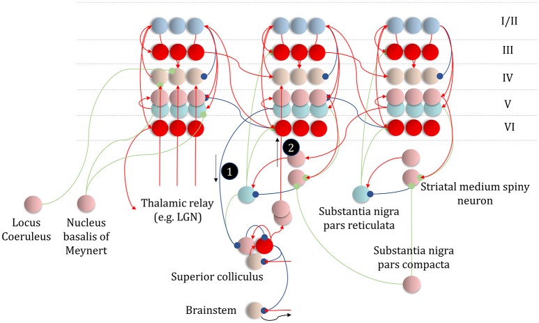
To infer the causes of its sensations, the brain must call on a generative (predictive) model. This necessitates passing local messages between populations of neurons to update beliefs about hidden variables in the world beyond its sensory samples. It also entails inferences about how we will act. Active inference is a principled framework that frames perception and action as approximate Bayesian inference. This has been successful in accounting for a wide range of physiological and behavioral phenomena. Recently, a process theory has emerged that attempts to relate inferences to their neurobiological substrates. In this paper, we review and develop the anatomical aspects of this process theory. We argue that the form of the generative models required for inference constrains the way in which brain regions connect to one another. Specifically, neuronal populations representing beliefs about a variable must receive input from populations representing the Markov blanket of that variable. We illustrate this idea in four different domains: perception, planning, attention, and movement. In doing so, we attempt to show how appealing to generative models enables us to account for anatomical brain architectures. Ultimately, committing to an anatomical theory of inference ensures we can form empirical hypotheses that can be tested using neuroimaging, neuropsychological, and electrophysiological experiments.

Keywords: Bayesian; active inference; generative model; message passing; neuroanatomy; predictive processing.


Figures

Figure 1
Figure 1
Forney factor graphs. The graphical model in this figure represents the (arbitrary) probability distribution shown below. Crucially, this distribution can be represented as the product of factors (ϕ) that represent prior and conditional distributions. By assigning each factor a square node, and connecting those factors that share random variables, we construct a graphical representation of the joint probability distribution. The “ = ” node enforces equality on all edges (lines) that connect to it. Small black squares represent observable data. This figure additionally illustrates a simple method for determining the Markov blanket of a variable (or set of variables). By drawing a line around all of the factor nodes connected to a variable, we find that the edges we intersect represent all of the constituents of the Markov blanket. For example, the green line shows that the blanket of w comprises x and v. The pink line shows the Markov blanket of v, which contains u, w, x, y, and z. The blue line indicates that v and z make up the blanket of y.
Figure 2
Figure 2
Partition functions and free energy. This schematic illustrates a useful operation known as “closing the box” or taking a partition function of part of a graph. By summing (or integrating) over all variables on edges within the dashed box, we can reduce this portion of the graph to a single factor that plays the part of a (marginal) likelihood. While it is not always feasible to perform the summation explicitly, we can approximate the marginal likelihood with a negative free energy. This affords an efficient method for evaluating subregions of the graph. Taking the partition function, or computing the free energy, for the whole graph allows us to evaluate the evidence sensory data affords the generative model.
Figure 3
Figure 3
Perception as inference. This figure shows two generative models that describe hidden state trajectories, and the data they generate. On the left, we show evolution of discrete states (s), represented as the “edges” (lines) connecting the square nodes, with probabilistic transitions B from one state to the next. Each of these states gives rise to a discrete observation (o), as determined by a likelihood mapping A. On the right, we show the analogous factor graph for continuous dynamics, in which states are described in terms of their positions (x), velocities (x′), accelerations (x″), etc., coupled by flows (f) (rates of change) and give rise to continuous observations (y) determined by a likelihood mapping (g). Numbered black circles indicate the messages that would need to be passed to infer the current state (left) or velocity (right). The equations below show how these could be combined to form a belief about these variables using two different inference schemes (variational message passing and belief propagation). That the same message passing architecture applies in both cases emphasizes the importance of the generative model and its Markov blankets. The precise form of these message passing schemes is unimportant from the perspective of this paper, but for technical details on variational message passing schemes, we refer readers to Winn and Bishop (2005), Dauwels (2007), and for belief propagation (Loeliger, ; Yedidia et al., 2005), and to the Appendix, which provides a brief outline of these schemes. Table 1 provides a short glossary for some of the mathematical notation used in this and subsequent figures.
Figure 4
Figure 4
The anatomy of perceptual inference. The neuronal network illustrated in this figure could be used to perform inferences about the model of Figure 3. Neurons in cortical layer IV represent the spiny stellate cells that receive input from relay nuclei of the thalamus, and from lower cortical areas. The appropriate thalamic relay depends upon the system in question. In the context of the visual system, it is the lateral geniculate nucleus (LGN). In the somatosensory or auditory systems, it is the ventral posterior nucleus or the medial geniculate nucleus, respectively. Layer IV cells in this network signal prediction errors, computed by comparing the optimal estimate (obtained by combining the messages from its Markov blanket) with the current belief, represented in superficial cortical layers. Assuming a logarithmic code (as in Figure 3), this involves subtracting (blue connection) the current estimates of the sufficient statistics from the sum (red connections) of the incoming messages. The numbered circles indicate the same messages as in Figure 3. We could also represent messages 4, 5, and 6 in exactly the same way.
Figure 5
Figure 5
Planning as inference. This figure illustrates the use of partition functions to evaluate regions of the graph (see also Figure 2). Crucially, while we can approximate a partition functions based upon past data using a free energy functional, we do not yet have data from the future. This means we instead need an expected free energy, to approximate the partition function under posterior predictive beliefs. The panel below the graph illustrates how we can re-express the expected free energy such that we can represent this portion of the graph in terms of two new factors: a marginal belief about future outcomes and a likelihood that becomes an expected entropy after taking the expectation. As G depends upon beliefs about outcomes, but not upon the outcomes themselves, we can compute this prior to observing data. In some accounts of active inference, this is made explicit by treating C as a prior that connects to a factor G (that acts as if it were a likelihood generating policies from outcomes). The circled numbers and letters here are consistent with those in Figure 6. For technical accounts of these equations, please see Friston et al. (2017d), Parr and Friston (2018c).
Figure 6
Figure 6
The basal ganglia. In the upper part of this figure, we show the same network as in Figure 4, but augmented such that it includes layer V cells encoding the gradients of the expected free energy and posterior predictive beliefs. These project to direct pathway medium spiny neurons and combine to give the expected free energy. This has a net inhibitory influence over the output nuclei (the globus pallidus internus and the substantia nigra pars reticulata), while the indirect pathway has a net excitatory effect. These are consistent with messages 2 and 3, respectively (the numbering is consistent with Figures 5, 7). Once the direct and indirect messages are combined at the globus pallidus internus, this projects via the thalamic fasciculus to the ventrolateral (VL) and ventral anterior nuclei of the thalamus. These modulate signals in the cortex, consistent with averaging beliefs about states under different policies, to compute average beliefs about the states (red neurons). Once we consider the hierarchical organization of this system (Figure 7), we need beliefs about preferences, derived from states at the higher level (message 3) combined with a posterior predictive belief (a) and an expected entropy term (b) to compute the gradient of the expected free energy. We additionally require a cortical input to the indirect pathway neurons, representing an empirical prior belief about policies (message 4—see Figure 7 for details). The coronal view of the basal ganglia, in the lower part of the figure, shows the connectivity of the direct (right) and indirect (left) pathways, to illustrate their consistency with the network above, but including the additional synapses that are not accounted for in the message passing. The substantia nigra pars compacta is included, and this modulates the weighting of messages 2 and 3. Please see the section below on Neuromodulation for details as to the emergence of dopaminergic phenomena from a generative model. In summary, the layers of the cortical microcircuit shown here represent beliefs about states under a given policy (I/II), beliefs about states averaged over policies (III), state prediction errors (IV), expected free energy gradients and predicted outcomes (V), and beliefs about states averaged over policies (VI).
Figure 7
Figure 7
Hierarchical models. This figure illustrates the extension of Figure 5 to two hierarchical levels; although this pattern could be recursively extended to an arbitrary number of levels. There are three points at which the levels interact. The first is a mapping from the outcomes of the higher level to the initial states at the lower level (A to “ = ” to B). An example of this might be a mapping from a sentence level representation to the first word of that sentence. The second associates higher level outcomes with low level empirical priors over policies (A to “ = ” to E). Finally, we allow the low-level preferences to depend upon higher level states (“ = ” to C).
Figure 8
Figure 8
Precision and uncertainty. This figure shows the graph of Figure 5, but supplemented with precision parameters and prior factors over these precisions. These encode confidence in policies (γ), transitions (ω), and likelihoods (ζ). The priors for these are the factors Γ, Ω, and Z, respectively. Note that the messages required to update beliefs about the hidden states are almost identical to those of Figure 3, but are now averaged over beliefs about the precision. Messages from the past (1) and future (2) are contextualized by the transition precision, while those from sensory input (3) are modulated by the likelihood precision. As in Figure 3, we provide the form of the variational and belief propagation messages implied by this model to illustrate the commonalities between their forms. Again, this is due to the structure of the Markov blankets of each state, which now includes precision parameters.
Figure 9
Figure 9
The anatomy of uncertainty. This schematic extends the network of Figure 6 to include modulatory variables, consistent with the factor graph of Figure 8. Specifically, we have now included subcortical regions that give rise to ascending neuromodulatory projections. This includes the locus coeruleus in the pons, which gives rise to noradrenergic signals. Axons from this structure travel through the dorsal noradrenergic bundle to reach the cingulum, a white matter bundle that allows dissemination of signals to much of the cortex. Here, we show these axons modulating messages 2 and 3, representing the past and future, respectively. The nucleus basalis of Meynert is the source of cholinergic signals to the cortex (again, via the cingulum). These modulatory connections target thalamocortical inputs to layer IV (i.e., message 1). Finally, the substantia nigra pars compacta (and the ventral tegmental area) projects via the medial forebrain bundle to the striatum, supplying it with dopaminergic terminals. This modulates the balance between prior and marginal likelihood influences over policy evaluation that we hypothesize correspond to indirect and direct pathway activity, respectively. As before, the layers of the cortical microcircuit shown here represent beliefs about states under a given policy (I/II), beliefs about states averaged over policies (III), state prediction errors (IV), expected free energy gradients and predicted outcomes (V), and beliefs about states averaged over policies (VI).
Figure 10
Figure 10
Decisions and movement. This graph illustrates how beliefs about categorical variables may influence those about continuous variables (message 1) and vice versa (message 2). The upper part of the graph is the same as that from Figure 5, while the lower part is that from the right of Figure 2. The additional η factor represents the empirical prior for a hidden cause, v, that determines the dynamics of x, much as the policies at the higher level determine the dynamics of state transitions. The equations below show that we can treat the descending message as a Bayesian model average, incorporating posterior predictive beliefs about outcomes under policies, averaged over policies. The ascending message is the free energy integrated over time for each outcome. This effectively treats each outcome as an alternative hypothesis for the continuous dynamics at the lower level.
Figure 11
Figure 11
An anatomy of inference. This schematic summarizes the networks we have discussed so far, but adds in the messages of Figure 10, with empirical priors propagated by message 1. These are subtracted from expectation neurons to give error signals, then used to update expectations. Expectations are used to derive predictions about sensory data. These are subtracted from the incoming data to calculate sensory errors, used to update current expectations, but also to drive brainstem reflexes through action (black arrow) to change sensory data (e.g., by moving the eyes). Message 2 derives from the expectations, which are used to compute the integral of the free energy over time. The relative evidence for each outcome is then propagated to layer IV cells in the cortex, acting as if it were sensory data. As before, the layers of the cortical microcircuit shown here represent beliefs about states under a given policy (I/II), beliefs about states averaged over policies (III), state prediction errors (IV), expected free energy gradients and predicted outcomes (V), and beliefs about states averaged over policies (VI).

Similar articles

Cited by

References

    1. Adams R. A., Perrinet L. U., Friston K. (2012). Smooth pursuit and visual occlusion: active inference and oculomotor control in Schizophrenia. PLoS ONE 7:e47502. 10.1371/journal.pone.0047502 - DOI - PMC - PubMed
    1. Adams R. A., Shipp S., Friston K. J. (2013). Predictions not commands: active inference in the motor system. Brain Struct. Funct. 218, 611–643. 10.1007/s00429-012-0475-5 - DOI - PMC - PubMed
    1. Aghajanian G. K., Marek G. J. (1999). Serotonin, via 5-HT2A receptors, increases EPSCs in layer V pyramidal cells of prefrontal cortex by an asynchronous mode of glutamate release. Brain Res. 825, 161–171. 10.1016/S0006-8993(99)01224-X - DOI - PubMed
    1. Albin R. L., Young A. B., Penney J. B. (1989). The functional anatomy of basal ganglia disorders. Trends Neurosci. 12, 366–375. 10.1016/0166-2236(89)90074-X - DOI - PubMed
    1. Andrews P. W., Bharwani A., Lee K. R., Fox M., Thomson J. A. (2015). Is serotonin an upper or a downer? The evolution of the serotonergic system and its role in depression and the antidepressant response. Neurosci. Biobehav. Rev. 51, 164–188. 10.1016/j.neubiorev.2015.01.018 - DOI - PubMed