Detecting neural assemblies in calcium imaging data

Abstract

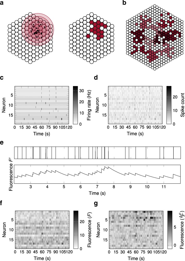
Background: Activity in populations of neurons often takes the form of assemblies, where specific groups of neurons tend to activate at the same time. However, in calcium imaging data, reliably identifying these assemblies is a challenging problem, and the relative performance of different assembly-detection algorithms is unknown.

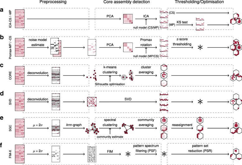
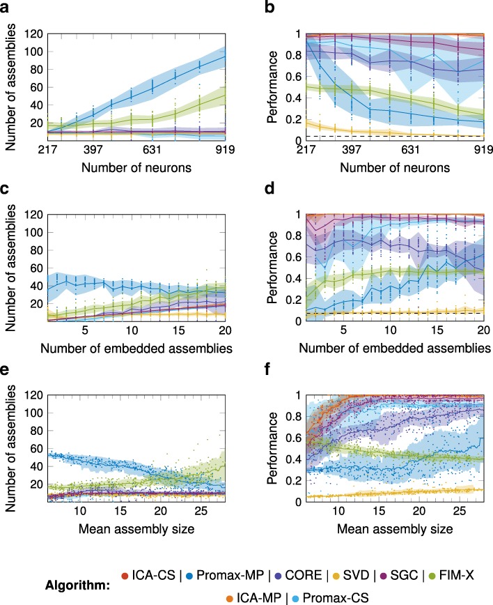
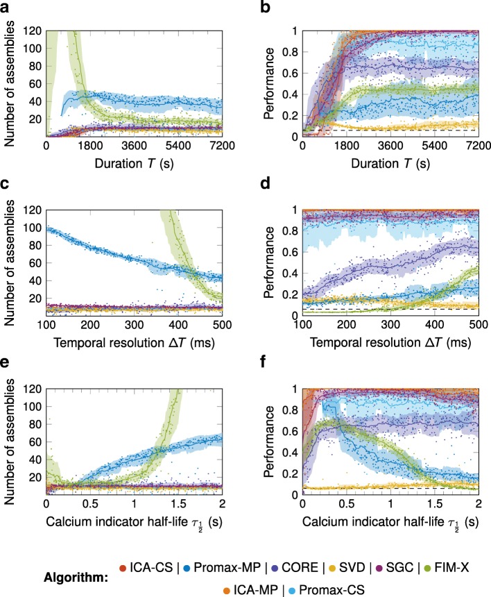
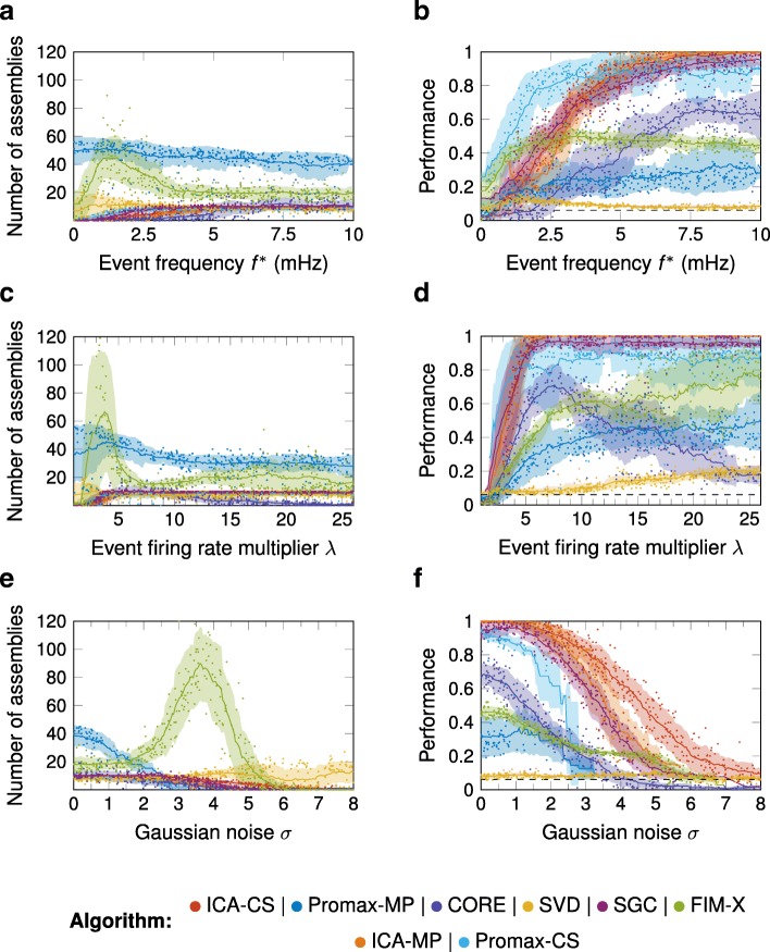
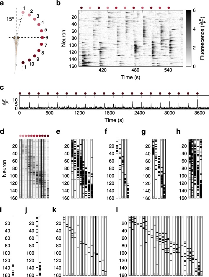
Results: To test the performance of several recently proposed assembly-detection algorithms, we first generated large surrogate datasets of calcium imaging data with predefined assembly structures and characterised the ability of the algorithms to recover known assemblies. The algorithms we tested are based on independent component analysis (ICA), principal component analysis (Promax), similarity analysis (CORE), singular value decomposition (SVD), graph theory (SGC), and frequent item set mining (FIM-X). When applied to the simulated data and tested against parameters such as array size, number of assemblies, assembly size and overlap, and signal strength, the SGC and ICA algorithms and a modified form of the Promax algorithm performed well, while PCA-Promax and FIM-X did less well, for instance, showing a strong dependence on the size of the neural array. Notably, we identified additional analyses that can improve their importance. Next, we applied the same algorithms to a dataset of activity in the zebrafish optic tectum evoked by simple visual stimuli, and found that the SGC algorithm recovered assemblies closest to the averaged responses.

Conclusions: Our findings suggest that the neural assemblies recovered from calcium imaging data can vary considerably with the choice of algorithm, but that some algorithms reliably perform better than others. This suggests that previous results using these algorithms may need to be reevaluated in this light.

Keywords: Clustering; Population coding; Spontaneous activity.

Fig. 1.

Generation of surrogate calcium imaging data. a On the left, points were drawn from a two-dimensional normal distribution, and a neuron was considered part of the assembly when at least one point fell within distance $\frac{1}{2}$ of its corresponding lattice point at its centre. The contour lines around the mean indicate regions of probability mass 50%, 90%, 99%, and 99.9%. The corresponding assembly is shown on the right. b An example of 10 assemblies (colour coded) embedded in a neural array of 469 neurons. Annuli represent neurons which overlap between two assemblies. c An example of the firing rates for 19 neurons over the course of 120 s. Neurons within the same assemblies simultaneously elevated their firing rates (here at 60 s, 77.5 s and 92 s). d The spike counts for the neurons over the course of 120 s as determined from independent Poisson random variables based on the firing rates shown in c. e The spiking events of a single neuron in a time-window of 10 s (top) and the corresponding calcium fluorescence after convolution with an exponential kernel (bottom). f The calcium fluorescence for the neurons over the course of 120 s. g The deflection of calcium fluorescence from baseline level, $\frac{\mathrm{\Delta F}}{F}$, for the neurons over the course of 120 s. This was the signal from which the algorithms attempted to reconstruct assembly structure

Fig. 2.

Schematics of the different algorithms investigated All algorithms can be divided into three phases: preprocessing, core assembly detection and thresholding/optimisation. a In the ICA algorithms, PCA is applied to $\frac{\mathrm{\Delta F}}{F}$, followed by ICA to the significant principal components. The null model for significance is either determined from circular shifts (ICA-CS) or given as the Marčenko-Pastur distribution (ICA-MP). The resulting principal components are either thresholded directly (ICA-CS) or after a KS test (ICA-MP) in order to arrive at the assemblies. b In the Promax algorithms, $\frac{\mathrm{\Delta F}}{F}$ is first reduced to its significant calcium transients, before PCA is applied. The null model for significant principal components is either given as the Marčenko-Pastur distribution (Promax-MP) or determined from circular shifts (Promax-CS). These principal components are rotated by means of Promax before z-score thresholding the components to arrive at the assemblies. c In the CORE algorithm, $\frac{\mathrm{\Delta F}}{F}$ is deconvolved and the resulting spike probabilities are thresholded into a binary signal. The activity patterns with a high level of activity are reduced to a set of core activity patterns (or ensembles) which are clustered using k-means clustering and the activity patterns of every community are averaged to arrive at the assemblies. d In the SVD algorithm, $\frac{\mathrm{\Delta F}}{F}$ is deconvolved and the resulting spike probabilities are thresholded into a binary signal. From the activity patterns with a high level of activity a similarity map is constructed and thresholded before SVD is applied. The assemblies were then inferred from the activity patterns corresponding to every significant singular vector. e In the SGC algorithm, $\frac{\mathrm{\Delta F}}{F}$ is thresholded to a binary signal and the activity patterns with a high level of activity are arranged into a graph according to their similarity. The graph is split into its communities using spectral clustering and the activity patterns of every community are averaged to arrive at the assemblies. f In the FIM-X algorithm, $\frac{\mathrm{\Delta F}}{F}$ is thresholded into a binary signal and FIM is applied to find co-active neurons as frequent item sets. These frequent item sets are reduced by PSF and PSR involving some additional statistical tests to arrive at the assemblies

Fig. 3.

Performance as a function of size of the neural array, number of embedded assemblies, and assembly size In every graph and for every algorithm the mean is depicted by a solid line together with the region of one standard deviation above and below. In the graphs for the performance, measured in terms of the Best Match score, the black dashed line indicates chance level of the Best Match score. a, b Varying the size of the neural array. With an increasing size of the neural array, Promax-MP and FIM-X detected an increasing number of assemblies and, consequently, their performance decreased. ICA-CS, ICA-MP, SGC, CORE, and SVD detected a constant number of assemblies and except for SVD showed good performance. Promax-CS performed well for smaller neural arrays, but slightly underestimated the number of assemblies in larger arrays. c, d Varying the number of embedded assemblies. Promax-MP detected an almost constant number of assemblies. ICA-CS, ICA-MP, SGC, Promax-CS, and FIM-X detected an increasing number of assemblies as the number of embedded assemblies increased, although FIM-X overestimated the total number. When there were only few assemblies embedded, Promax-CS underestimated the total number, while when there were more assemblies embedded, CORE overestimated and SVD underestimated the total number. e, f Varying the assembly sizes. ICA-CS, ICA-MP, SGC, Promax-CS, CORE, and SVD detected a constant number of assemblies except when the embedded assemblies were particularly small. Promax-MP and FIM-X overestimated the number of assemblies

Fig. 4.

Performance as a function of simulation duration, temporal resolution, and calcium indicator half-life Graphing conventions as in Fig. 3. a, b Varying the simulation duration T. With increasing T, the performance of ICA-CS, ICA-MP, SGC and Promax-CS increased and they detected a constant number of assemblies beyond T=1800s. Promax-MP overestimated the total number, and the number detected by FIM-X showed a steep peak, while SVD underestimated the total number. c, d Varying the temporal resolution ΔT. With increasing ΔT, Promax-MP and FIM-X detected a decreasing number of assemblies. They both overestimated the total number, particularly FIM-X at small ΔT. SVD underestimated the total number of assemblies. ICA-CS, ICA-MP, SGC, Promax-CS and CORE detected a constant number of assemblies and ICA-CS, ICA-MP, SGC and Promax-CS also showed good performance. e, f Varying the calcium indicator half-life ${\tau }_{\frac{1}{2}}$. With increasing ${\tau }_{\frac{1}{2}}$ Promax-MP and FIM-X detected an increasing number of assemblies. ICA-CS, ICA-MP, SGC, Promax-CS, CORE and SVD detected a constant number of assemblies and ICA-CS, ICA-MP, SGC, Promax-CS and CORE showed good performance

Fig. 5.

Performance as a function of the event frequency, event firing rate multiplier, and the standard deviation of the noise Graphing conventions as in Fig. 3. a, b Varying the event frequency f^∗. With increasing f^∗, the performance of ICA-CS, ICA-MP, SGC, Promax-CS and CORE increased and they detected a constant number of assemblies beyond f^∗=5mHz. At low frequencies the performance of Promax-CS exceeded that of ICA-CS, ICA-MP and SGC. Promax-MP and FIM-X both overestimated the number of assemblies. c, d Varying the event firing rate multiplier λ. With increasing λ, the performance of ICA-CS, ICA-MP, SGC, and Promax-CS increased and, when λ exceeded about 4, they detected a constant number of assemblies and showed good performance. Promax-MP and FIM-X both overestimated the number of assemblies. The performance of CORE first increased but then consequently decreased as it underestimated the total number of assemblies. e, f Varying the standard deviation σ of the Gaussian noise. With increasing σ, every algorithm (except FIM-X, which instead showed a peak, and SVD) detected a decreasing number of assemblies and, consequently, their performance decreased. For noise levels beyond σ=3 neither Promax-MP or Promax-CS yielded any results since they were not able to fit the noise model to the data

Fig. 6.

Application of the different algorithms to stimulus-evoked calcium imaging data from the larval zebrafish optic tectum. a 11 different stimuli were shown to the fish. The stimuli were separated by 15° in the visual field of the fish. b The deflection of calcium fluorescence from baseline level, $\frac{\mathrm{\Delta F}}{F}$, for the 160 neurons over about 180 s of the recording. The neurons are ordered by their anterior-posterior position in the tectum. The stimuli were presented in the order 11 – 1 – 10 – 2 – 6 – 3 – 8 – 4 – 9 – 5 – 7 as indicated. c Example calcium trace over the course of the whole experiment from a neuron particularly responsive to stimulus 11, whose onset is indicated. The overall noise is relatively low and the peaks in fluorescence are clearly visible. d The average population response in terms of fluorescence ($\frac{\mathrm{\Delta F}}{F}$) to the 11 different stimuli. The responses to the first 3 stimuli were weak compared to the others. e–j Graphical representations of the assemblies recovered by the different algorithms. The neurons which were part of the respective assemblies are marked in black. e SGC recovered 8 assemblies. f ICA-CS recovered 5 assemblies. g Promax-CS recovered 5 assemblies. h SVD recovered 5 assemblies. i CORE recovered 1 assembly. j ICA-MP recovered 2 assemblies. k Promax-MP recovered 16 assemblies. l FIM-X recovered 27 assemblies

References

1. Gerstein G.L., Bedenbaugh P., Aertsen A.M.H.J. Neuronal assemblies. IEEE Transactions on Biomedical Engineering. 1989;36(1):4–14. doi: 10.1109/10.16444. - DOI - PubMed
1. Sakata Shuzo, Harris Kenneth D. Laminar Structure of Spontaneous and Sensory-Evoked Population Activity in Auditory Cortex. Neuron. 2009;64(3):404–418. doi: 10.1016/j.neuron.2009.09.020. - DOI - PMC - PubMed
1. Truccolo Wilson, Hochberg Leigh R, Donoghue John P. Collective dynamics in human and monkey sensorimotor cortex: predicting single neuron spikes. Nature Neuroscience. 2009;13(1):105–111. doi: 10.1038/nn.2455. - DOI - PMC - PubMed
1. Berkes P., Orban G., Lengyel M., Fiser J. Spontaneous Cortical Activity Reveals Hallmarks of an Optimal Internal Model of the Environment. Science. 2011;331(6013):83–87. doi: 10.1126/science.1195870. - DOI - PMC - PubMed
1. Hyman J. M., Whitman J., Emberly E., Woodward T. S., Seamans J. K. Action and Outcome Activity State Patterns in the Anterior Cingulate Cortex. Cerebral Cortex. 2012;23(6):1257–1268. doi: 10.1093/cercor/bhs104. - DOI - PubMed
Publication types
LinkOut - more resources