Self-organising coordinate transformation with peaked and monotonic gain modulation in the primate dorsal visual pathway

Abstract

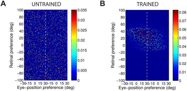
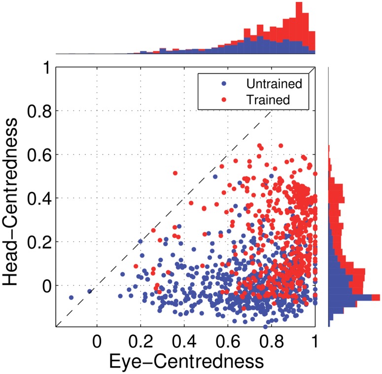
We study a self-organising neural network model of how visual representations in the primate dorsal visual pathway are transformed from an eye-centred to head-centred frame of reference. The model has previously been shown to robustly develop head-centred output neurons with a standard trace learning rule, but only under limited conditions. Specifically it fails when incorporating visual input neurons with monotonic gain modulation by eye-position. Since eye-centred neurons with monotonic gain modulation are so common in the dorsal visual pathway, it is an important challenge to show how efferent synaptic connections from these neurons may self-organise to produce head-centred responses in a subpopulation of postsynaptic neurons. We show for the first time how a variety of modified, yet still biologically plausible, versions of the standard trace learning rule enable the model to perform a coordinate transformation from eye-centred to head-centred reference frames when the visual input neurons have monotonic gain modulation by eye-position.

Fig 1. Architecture of the neural network model.

The competitive output layer on the right receives afferent synaptic connections from neurons in the input layer on the left. A trace learning rule is used to modify the strengths of the feedforward synaptic connections from the input layer to the output layer during learning.

Fig 2. Examples of the two alternative response functions used to compute the firing rates of input neurons.

For each type of response function, we plot the responses of an individual input neuron as a function of eye-position and retinal location of a visual target. A: Example of a peaked response function, in which the firing rate is modulated by a peaked eye-position gain field as described by Eq 1. B: Example of a monotonic response function that is modulated by a sigmoidal eye-position gain field described by Eq 2.

Fig 3. Comparison of model performance with peaked and sigmoidal (monotonic) gain modulation of visual input neurons.

The figure shows the firing rate responses of output neurons before and after training with the standard trace rule (6). Specifically, each subplot shows the firing rate responses of a typical output neuron during testing for four different eye-positions: −18°, −6°, 6° and 18°. The top row shows output neuron #95 from the model with peaked eye-position gain modulation before training (A) and after training (B). The bottom row shows output neuron #838 from the model with sigmoidal eye-position modulation before training (C) and after training (D). In each subplot, each curve corresponds to a fixed eye-position while a visual target is presented across the same range of head-centred locations. It is evident in subplot (B) that after training the model with peaked gain modulation of the input neurons, the output neuron responds reasonably consistently when the visual target is presented within the localised interval of head-centred space [0°, 16°] regardless of the eye-position. The neuron is thus responding in a head-centred reference frame. However, in contrast, subplot (D) shows that after training the model with sigmoidal (monotonic) gain modulation, the responses of the output neuron in the head-centred visual space are much more dependent on the eye-position. Thus, this neuron is not representing the target position in a head-centred reference frame. The miniature scatter plots show the reference frame values of all neurons in the output layer, where each neuron is plotted as a point corresponding to that neuron’s particular combination of head-centredness (ordinate) and eye-centredness (abscissa). The neuron whose firing rate responses have been plotted is shown in the scatter plot by a red mark. The miniature scatter plots confirm the same general effects across the entire populations of output neurons. That is, subplot (B) shows that a large proportion of the output neurons are clustered in the top left quadrant of the scatter plot, indicating a high head-centredness (ordinate) and low eye-centredness (abscissa). These output neurons are thus responding in a head-centred frame of reference. While subplot (D) shows that a large proportion of the output neurons are clustered in the bottom right quadrant of the scatter plot, indicating a low head-centredness (ordinate) and high eye-centredness (abscissa). Thus, with monotonic gain fields acting on the input neurons, the population of output neurons have overwhelmingly learned to respond in an eye-centred reference frame.

Fig 4. Strengths of the afferent synapses from the input population to a typical output neuron during testing.

Results are shown for the model with peaked eye-position gain modulation before training (A) and after training (B), and for the model with sigmoidal eye-position modulation before training (C) and after training (D). The output neurons correspond to those plotted in Fig 3. In each plot, the afferent synapses have been arranged topographically by the preference of the input neuron for retinal location α_i and eye-position β_j. For the model with sigmoidal gain modulation, there are two input neurons for every combination of retinal preference and eye-position preference, but with opposite eye-position gain. Consequently, the input population has been separated by gain direction. The portion of each plot to the left of the white dashed line corresponds to input neurons with positive gain κ_j > 0, while the portion of each plot to the right of the white dashed line corresponds to those input neurons with negative gain κ_j < 0. It can be seen from subplot (B) that the output neuron in the trained network with peaked gain modulation has developed a diagonal weight structure, which is consistent with a learned response to a particular location within the head-centred frame of reference. In contrast, subplot (D) shows that the output neuron in the trained network with sigmoidal (monotonic) gain modulation has developed a more horizontal weight structure, which is consistent with a learned response to a specific location within the eye-centred reference frame.

Fig 5. Scatter plot of eye-centredness and head-centredness values of output neurons from simulations with peaked and monotonic gain modulation.

The scatter plot shows the eye-centredness and head-centredness values of all output neurons from four separate simulations corresponding to the models with peaked and sigmoidal (monotonic) gain modulation tested before and after training with the standard trace rule (Eq 6). Each point in the scatter plot corresponds to an output neuron from the given simulation, plotted in terms of its eye-centredness (abscissa) and head-centredness (ordinate). The dashed diagonal line with positive unity slope separates those neurons which are classified as head-centred (above line) from those that are classified as eye-centred (below the line). It is evident that after training most of the output neurons from the network with peaked gain modulation have become head-centred, while nearly all of the output neurons from the network with monotonic gain modulation have remained eye-centred.

Fig 6. Covariance between a given input neuron and the rest of the input neuron population.

Each plot shows the covariance between a given input neuron and the rest of the input neuron population in the form of a topographic map analogous to the weight vector maps shown above. Subplots (A) and (B) show results for input neurons with peaked and monotonic gain, respectively. In both cases the input neuron has preferences α = β = 0°, and in the monotonic case the input has positive gain (κ > 0).

Fig 7. Weight vectors of two typical output neurons.

The top row shows the weight vectors of two typical output neurons that develop when the input neurons have peaked eye-position gain modulation and the network is trained with either the Hebbian learning rule (A) or the trace learning rule (B). The bottom row shows the weight vectors of two typical output neurons when the input neurons have monotonic eye-position gain and the network is trained with either the Hebbian learning rule (C) or the standard trace learning rule (D).

Fig 8. Synaptic weight structure of a network model that has been manually prewired in order to produce head-centred output neurons with input neurons that are modulated by a sigmoidal function of eye-position.

The figure shows the structure of the canonical weight vector resulting from the prewiring Eqs 14 and 15. Each of the two rectangles represents the topographic organisation of one half of the input population in terms of retinal-preference (α_i) and eye-position preference (β_j), with the input neurons in the left rectangle having κ > 0 (positive gain) and the right rectangle having κ < 0 (negative gain). A neuron in the competitive output population which has been assigned a head-centred receptive field at location h will have elevated connections from input neurons with preferences located in the right-angled triangles of the input space, labeled A and B.

Fig 9. Performance of the prewired network model with monotonic modulated input neurons.

The Figure shows the performance of the network model that has been manually prewired to produce head-centred output neurons with input neurons that are modulated by a sigmoidal function of eye-position. The scatter plot shows the eye-centredness and head-centredness values of all output neurons from the manually prewired model and a randomly wired model. Same conventions as in Fig 5. It can be seen that the majority of the output neurons in the manually prewired model display head-centred responses.

Fig 10. The effects of introducing synaptic plasticity into the network that has been manually prewired to produce head-centred output neurons when the input neurons that are modulated by a sigmoidal (monotonic) function of eye-position.

The figure shows population analyses of the response properties of output neurons in the manually prewired model as the synaptic weights are further modified during ten training epochs with the standard trace learning rule (6). Three key summary statistics are given. The head-centredness rate (red) is the fraction of head-centred neurons in the output population. The average head-centredness (green) is the average head-centredness among head-centred neurons, and becomes undefined if no head-centred neurons are found to exist. The average eye-centredness (blue) is the average eye-centredness among all output neurons. The dashed lines show these values for the manually prewired network before training, while the unbroken lines show the values through successive training epochs after synaptic plasticity has been introduced. The error bars are the standard deviations. It can be seen that by the end of the first training epoch the majority of the output neurons switched from being head-centred to eye-centred.

Fig 11. The effects of incorporating a mixed population of input neurons with both peaked and monotonic eye-position gain modulation.

The plots show how the performance metrics vary with the monotonic modulation rate, p, which is the probability of each input neuron having a monotonic eye-position gain modulation. Results are presented showing the response characteristics of the output neurons before training (A) and after training (B). Conventions are similar to Fig 10. It is evident that the head-centredness rate decreased as the sigmoid modulation rate increased, both in the trained and untrained models. However, as long as the sigmoid modulation rate is less than 30%, the trained model had a higher proportion of head-centred output neurons than the untrained model.

Fig 12. Simulation results showing the firing rate responses of a model incorporating a population of monotonic modulated input neurons trained with the modified learning rule 16: Delayed postsynaptic trace with anti-Hebbian learning.

The figure shows the firing rate responses of output neuron #168 before training (A) and after training (B) during testing for four different eye-positions: −18°, −6°, 6° and 18°. In each subplot, each curve corresponds to a fixed eye-position while a visual target is presented across the same range of head-centred locations. The miniature scatter plot shows the reference frame values of all neurons in the output layer, where each neuron is plotted as a point corresponding to that neuron’s particular combination of head-centredness (ordinate) and eye-centredness (abscissa). The neuron whose firing rate responses have been plotted is shown in the scatter plot by a red mark. After training it is evident that this neuron responds reasonably invariantly to a visual target presented at the same head-centred location regardless of the eye-position.

Fig 13. Simulation results showing the strengths of the afferent synapses of a model incorporating a population of sigmoidal modulated input neurons trained with the modified learning rule 16: Delayed postsynaptic trace with anti-Hebbian learning.

The figure shows the strengths of the afferent synapses from the input population to output neuron #168 for the untrained (A) and trained (B) model. The output neuron corresponds to the one plotted in Fig 12. In each plot, the afferent synapses have been arranged topographically by the preference of the input neuron for retinal location α_i and eye-position β_j. The portion of each plot to the left of the white dashed line corresponds to input neurons with positive gain κ_j > 0, whilst the portion of each plot to the right of the white dashed line corresponds to those input neurons with negative gain κ_j < 0. The synaptic weights for this output neuron after training (B) have approximately the correct structure for a head-centred neuron as shown in Fig 8.

Fig 14. Simulation results showing the output reference frame response characteristics of a model incorporating a population of sigmoidal modulated input neurons trained with the modified learning rule 16: Delayed postsynaptic trace with anti-Hebbian learning.

The scatter plot shows the reference frame response characteristics of all output neurons before and after training. Each neuron is represented as a point corresponding to its combination of eye-centredness (abscissa) and head-centredness (ordinate) values. Data points for the untrained model are plotted in blue and data points for the trained model are shown in red. The dashed diagonal line with positive unity slope separates those neurons which are classified as head-centred (above the line) from those that are classified as eye-centred (below the line). It can be seen that many of the output neurons have developed head-centred output responses after training.

Fig 15. Simulation results showing the firing rate responses of a model incorporating a population of monotonic modulated input neurons trained with the modified learning rule 18: Delayed postsynaptic firing rate with anti-Hebbian learning.

The figure shows the firing rate responses of output neuron #876 before training (A) and after training (B) during testing for four different eye-positions: −18°, −6°, 6° and 18°. Conventions as for Fig 12. The comparison of subplot (A) and subplot (B) shows that the output neuron learned to respond to a specific head-centred location regardless of the eye-position after training.

Fig 16. Simulation results showing the strengths of the afferent synapses of a model incorporating a population of sigmoidal modulated input neurons trained with the modified learning rule 18: Delayed postsynaptic firing rate with anti-Hebbian learning.

The figure shows the strengths of the afferent synapses from the input population to output neuron #876 for the untrained (A) and trained (B) model. The output neuron corresponds to the one plotted in Fig 15. Conventions as for Fig 13. The synaptic weight structure for this output neuron after training shown in plot (B) has approximately the correct profile for a head-centred neuron (Fig 8).

Fig 17. Simulation results showing the output reference frame response characteristics of a model incorporating a population of sigmoidal modulated input neurons trained with the modified learning rule 18: Delayed postsynaptic firing rate with anti-Hebbian learning.

The scatter plot shows the reference frame response characteristics of all output neurons before and after training. Conventions as for Fig 14. It is evident that training had the effect of increasing the head-centredness values of most output neurons. Indeed many more head-centred output neurons are present in the trained model than in the untrained model.

Fig 18. Simulation results showing the firing rate responses of a model incorporating a population of monotonic modulated input neurons trained with the modified learning rule 19: Current postsynaptic trace with anti-Hebbian learning.

The figure shows the firing rate responses of output neuron #328 before training (A) and after training (B) during testing for four different eye-positions: −18°, −6°, 6° and 18°. Conventions as for Fig 12. The comparison of subplot (A) and subplot (B) shows that the output neuron learned to respond to a specific head-centred location regardless of the eye-position after training.

Fig 19. Simulation results showing the strengths of the afferent synapses of a model incorporating a population of sigmoidal modulated input neurons trained with the modified learning rule 19: Current postsynaptic trace with anti-Hebbian learning.

The figure shows the strengths of the afferent synapses from the input population to output neuron #328 for the untrained (A) and trained (B) model. The output neuron corresponds to the one plotted in Fig 18. Conventions as for Fig 13. The synaptic weight structure for this output neuron after training shown in plot (B) has the correct kind of profile for a head-centred neuron (Fig 8).

Fig 20. Simulation results showing the output reference frame response characteristics of a model incorporating a population of sigmoidal modulated input neurons trained with the modified learning rule 19: Current postsynaptic trace with anti-Hebbian learning.

The scatter plot shows the reference frame response characteristics of all output neurons before and after training. Conventions as for Fig 14. It can be seen that training increased the head-centredness values of most output neurons, with quite a number of head-centred output neurons present in the trained model.

Fig 21. Simulation results showing the firing rate responses of a model incorporating a population of monotonic modulated input neurons trained with the modified learning rule 20: Delayed postsynaptic trace learning rule.

The figure shows the firing rate responses of output neuron #223 before training (A) and after training (B) during testing for four different eye-positions: −18°, −6°, 6° and 18°. Conventions as for Fig 12. The comparison of subplot (A) and subplot (B) shows that the output neuron learned to respond to a specific head-centred location regardless of the eye-position after training. Output neuron #223 is not shown in the scatter plot of subplot (A) because this neuron did not respond for every eye-position before training and was therefore excluded from further analysis (section Analysis of Network Performance). However, subplot (B) shows that the same output neuron learned to respond to a specific head-centred location regardless of the eye-position after training.

Fig 22. Simulation results showing the strengths of the afferent synapses of a model incorporating a population of sigmoidal modulated input neurons trained with the modified learning rule 20: Delayed postsynaptic trace learning rule.

The figure shows the strengths of the afferent synapses from the input population to output neuron #223 for the untrained (A) and trained (B) model. The output neuron corresponds to the one plotted in Fig 21. Conventions as for Fig 13. The synaptic weight structure for this output neuron after training shown in plot (B) has approximately the correct profile for a head-centred neuron (Fig 8).

Fig 23. Simulation results showing the output reference frame response characteristics of a model incorporating a population of sigmoidal modulated input neurons trained with the modified learning rule 20: Delayed postsynaptic trace learning rule.

The scatter plot shows the reference frame response characteristics of all output neurons before and after training. Conventions as for Fig 14. It is evident that training had the effect of increasing the head-centredness values of most output neurons. Although, there is only a single head-centred output neuron present in the trained model.

Fig 24. Simulation results of a model incorporating a mixed population of peaked and sigmoidal modulated input neurons, with sigmoidal modulation rate p set to 0.5, trained with the modified learning rule 20: Delayed postsynaptic trace learning rule.

The figure shows the firing rate responses of output neuron #281 before training (A) and after training (B) during testing for four different eye-positions: −18°, −6°, 6° and 18°. Conventions as for Fig 12. Plot (B) shows that the same output neuron learned to respond to a specific head-centred location regardless of the eye-position after training.

Fig 25. Simulation results of a model incorporating a mixed population of peaked and sigmoidal modulated input neurons, with sigmoidal modulation rate p set to 0.5, trained with the modified learning rule 20: Delayed postsynaptic trace learning rule.

The figure shows the strengths of the afferent synapses from the input population to output neuron #281 for the untrained (A) and trained (B) model. The output neuron corresponds to the one plotted in Fig 24. Conventions as for Fig 13. The synaptic weight structure for this output neuron after training shown in plot (B) has the correct kind of profile for a head-centred neuron (Fig 8).

Fig 26. Simulation results of a model incorporating a mixed population of peaked and sigmoidal modulated input neurons, with sigmoidal modulation rate p set to 0.5, trained with the modified learning rule 20: Delayed postsynaptic trace learning rule.

The scatter plot shows the reference frame response characteristics of all output neurons before and after training. Conventions as for Fig 14. It is evident that training had the effect of increasing the head-centredness values of most output neurons, with many more head-centred output neurons present in the trained model.

References

1. Andersen RA, Mountcastle VB. The influence of the angle of gaze upon the excitability of the light-sensitive neurons of the posterior parietal cortex. The Journal of Neuroscience. 1983;3(3):532–548. 10.1523/JNEUROSCI.03-03-00532.1983 - DOI - PMC - PubMed
1. Andersen R, Essick G, Siegel R. Encoding of spatial location by posterior parietal neurons. Science. 1985;230(4724):456–458. 10.1126/science.4048942 - DOI - PubMed
1. Andersen R, Bracewell R, Barash S, Gnadt J, Fogassi L. Eye position effects on visual, memory, and saccade-related activity in areas LIP and 7a of macaque. The Journal of Neuroscience. 1990;10(4):1176–1196. 10.1523/JNEUROSCI.10-04-01176.1990 - DOI - PMC - PubMed
1. Galletti C, Battaglini P, Fattori P. Eye Position Influence on the Parieto-occipital Area PO of the Macaque Monkey. European Journal of Neuroscience. 1995;7(12):2486–2501. 10.1111/j.1460-9568.1995.tb01047.x - DOI - PubMed
1. Mullette-Gillman OA, Cohen YE, Groh JM. Eye-Centered, Head-Centered, and Complex Coding of Visual and Auditory Targets in the Intraparietal Sulcus. Journal of Neurophysiology. 2005;94(4):2331–2352. 10.1152/jn.00021.2005 - DOI - PubMed
Publication types