Hierarchy of speech-driven spectrotemporal receptive fields in human auditory cortex

Abstract

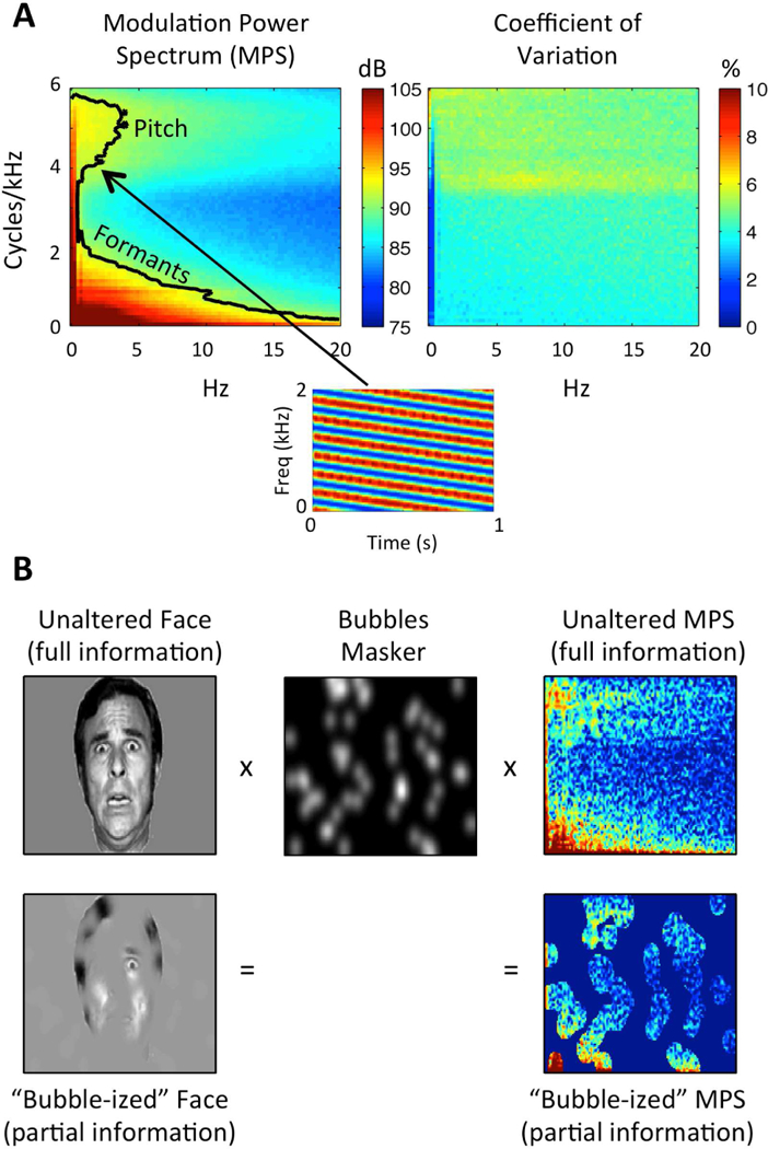
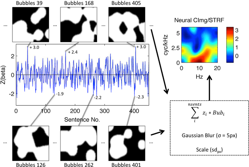
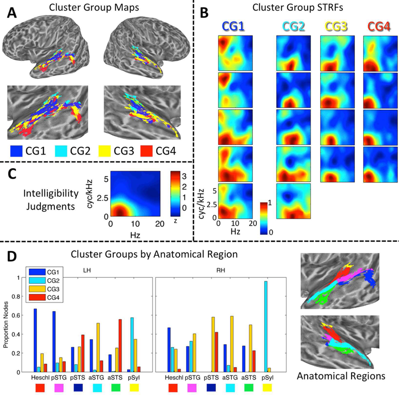
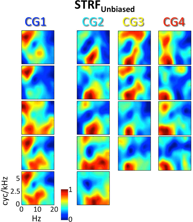
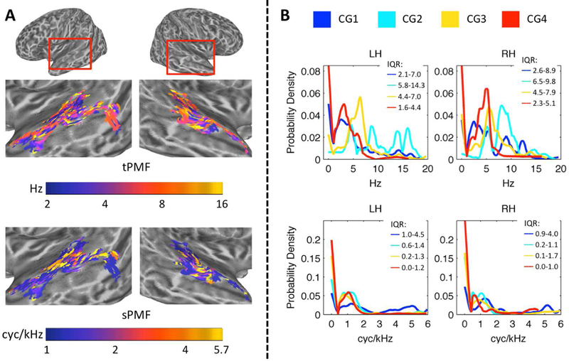
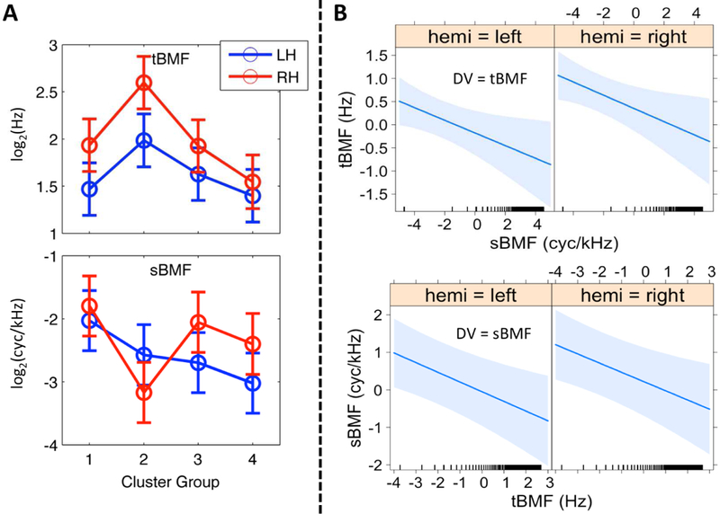
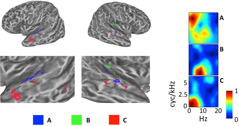
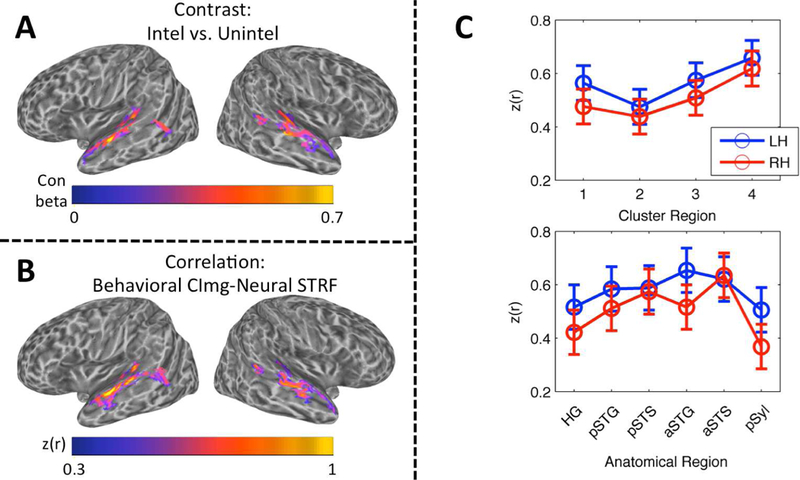
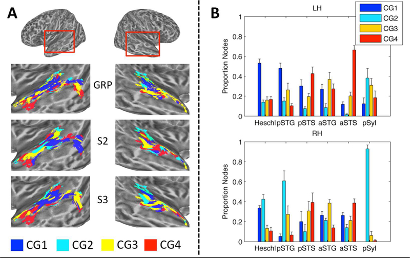
Existing data indicate that cortical speech processing is hierarchically organized. Numerous studies have shown that early auditory areas encode fine acoustic details while later areas encode abstracted speech patterns. However, it remains unclear precisely what speech information is encoded across these hierarchical levels. Estimation of speech-driven spectrotemporal receptive fields (STRFs) provides a means to explore cortical speech processing in terms of acoustic or linguistic information associated with characteristic spectrotemporal patterns. Here, we estimate STRFs from cortical responses to continuous speech in fMRI. Using a novel approach based on filtering randomly-selected spectrotemporal modulations (STMs) from aurally-presented sentences, STRFs were estimated for a group of listeners and categorized using a data-driven clustering algorithm. 'Behavioral STRFs' highlighting STMs crucial for speech recognition were derived from intelligibility judgments. Clustering revealed that STRFs in the supratemporal plane represented a broad range of STMs, while STRFs in the lateral temporal lobe represented circumscribed STM patterns important to intelligibility. Detailed analysis recovered a bilateral organization with posterior-lateral regions preferentially processing STMs associated with phonological information and anterior-lateral regions preferentially processing STMs associated with word- and phrase-level information. Regions in lateral Heschl's gyrus preferentially processed STMs associated with vocalic information (pitch).

Keywords: Bubbles; Classification images; Spectrotemporal modulations; Speech perception; fMRI.

Figure 1.

(A) Speech Modulation Power Spectrum. Left: Average MPS of 452 sentences spoken by a single female talker. The MPS describes speech as a weighted sum of spectrotemporal ripples containing energy at a unique combination of temporal (Hz; abscissa) and spectral (cycles/kHz; ordinate) modulation rate. Modulation energy (dB, arb. ref; color scale) clusters into two discrete regions: a high-spectral-modulation-rate region corresponding to finely spaced harmonics of the fundamental (a “pitch region”) and a low-spectral-modulation-rate region corresponding to coarsely spaced resonant frequencies of the vocal tract (a “formant region”). The black contour line indicates the modulations accounting for 80% of the total modulation power. A spectrogram of an example spectrotemporal ripple (2 Hz, 4 cyc/kHz) is shown beneath. Right: Coefficient of variation across the 452 sentences (sd/mean), expressed as a percentage (color scale). Plotted on the same axes as the MPS. There is relatively little variation across utterances (maximum CV ~7%). (B) Bubbles Procedure. Bubbles (middle) are applied to an image of a face (left) and the MPS of an individual sentence (right). In either case, bubbles reduce the information in the stimulus. Different random bubble patterns are applied across trials of an experiment. For auditory bubbles, we in practice use a binary masker with bubbles that are larger than those shown in the example.

Figure 2.. Bubbles Analysis Schematic.

A BOLD activation time-course from a single voxel in left Heschl’s gyrus of a representative subject is shown (blue line). The time-course plots the z-scored time-series of single-trial activation magnitudes (beta; ordinate) evoked by “bubble-ized” sentences (Sentence No., abscissa). Example bubble patterns (black-and-white panels) associated with sentences that evoked relatively large (top) and small (bottom) activations are plotted and identified by their sentence number. Z-scored activation magnitudes associated with these examples are shown next to the corresponding point in the activation time-course. Bubbles are applied to the MPS of each sentence as shown in Fig. 1. White pixels show regions of the MPS that are transmitted to the listener, while black pixels show regions of the MPS that are removed. Each bubble pattern is multiplied by its associated z-score, and the series of bubble patterns is summed pixel-by-pixel. The resulting summed image is then blurred (Gaussian filter with sigma = 5 pixels) and scaled by the across-pixel standard deviation (sd_px). The result is a STRF (top right) showing which regions of the MPS best activated this voxel. The STRF color scale is in across-pixel standard deviation units, where large positive values (yellow-red) correspond to regions of the MPS that evoked relatively large activations.

Figure 3.

(A) Maps of STRF Cluster Groups in Auditory Cortex. Cluster Groups are plotted by color on cortical surface renderings of the left and right hemispheres. Zoomed renderings of the temporal lobe are shown beneath whole-brain plots. Cluster Group 1 (CG1, blue) is located primarily in the supratemporal plane and posterior STG. Cluster Group 2 (CG2, cyan) is located primarily in medial supratemporal reigons. Cluster Groups 3 and 4 (CG3/4, yellow/red) are located primarily in the posterior and anterior STG/STS. (B) STRF-Cluster Patterns. For each of the 18 STRF clusters identified by GMM analysis, the cluster-average group-level (t-score) STRF is plotted. STRF magnitudes have been normalized to the range [0, 1]. Larger values are associated with STMs that produced relatively more BOLD activation. STRFs are organized by Cluster Group (CG1–4) in columns running from left to right. STRFs associated with CG1 respond to a broad range of STMs. STRFs associated with CG2 respond especially to high temporal modulation rates. STRFs associated with CG3/4 respond to STMs important for intelligibility (see C). (C) Behavioral Classification Image for Intelligibility Judgments. This plot is essentially a ‘behavioral STRF’, derived entirel y from button-press responses (yes-no intelligibility judgments) rather than neural activity. The z-scored group-level behavioral classification image is shown. Larger values are associated with STMs that contribute relatively more to intelligibility. Temporal modulations from 2–7 Hz and spectral modulations less than 1 cyc/kHZ contribute maximally.(D) Distribution of Cluster Groups within Anatomically Defined Regions. The proportion of cortical surface nodes belonging to CG1–4 is plotted for six anatomical regions of interest in the left (LH) and right (RH) hemispheres: Heschl = Heschl’s gyrus/sulcus, pSTG/S = posterior STG/S, aSTG/S = anterior STG/S, pSyl = posterior Sylvian cortex. Colored boxes beneath region labels correspond to the colors of the anatomical regions plotted on zoomed cortical surface renderings at right. Only significantly tuned cortical surface nodes are labeled.

Figure 4.. Cluster level STRFs with the global effect of intelligibility removed (STRF_Unbiased).

For each of the 18 STRF clusters identified by GMM analysis, the cluster-average group-level (t-score) STRF_Unbiased is plotted. STRF magnitudes have been normalized to the range [0, 1]. Larger values are associated with STMs that produced relatively more BOLD activation. STRFs are organized by Cluster Group (CG1–4) in columns running from left to right. Compare to Fig. 3B.

Figure 5.

(A) Cortical Maps of Peak Modulation Frequencies. Node-wise maps of temporal peak modulation frequency (tPMF, Hz) and spectral peak modulation frequency (sPMF, cyc/kHz) are displayed on inflated cortical surface renderings of the left and right temporal lobes. The renderings have been zoomed in as indicated by the red boxes at the top of the figure. Color scales are logarithmic. (B) Probability Density of tPMF and sPMF Within Cluster Groups. Empirical cumulative distribution functions (eCDFs; Kaplan-Meier method) for tPMF (Hz, top) and sPMF (cyc/kHz, bottom) were generated. Empirical probability density functions (ePDFs) were obtained by taking the derivative of the eCDFs. The ePDFs are plotted for each cluster group (colored lines, see legend) separately for the left (LH) and right (RH) hemispheres. The interquartile ranges (25^th percentile – 75^th percentile) of each distribution are indicated at the top right of each panel (IQR). The ordinate is the estimated probability density.

Figure 6.. Linear Mixed Effects Models: Best Modulation Frequency.

(A) Effect of Cluster Region. The mean of the fitted values produced by the LME model for temporal (tBMF, top) and spectral (sBMF, bottom) best modulation frequencies (octave scale, ordinate) are plotted for Cluster Groups 1–4 (abscissa) in the left (blue) and right (red) hemispheres. Error bars reflect ± 1 SEM. Spectral BMFs are negative because nodes with an sBMF of 0, of which there were many, were set to 0.01 (−6.6 on the octave scale). (B) Covariation between tBMF and sBMF. Results of linear mixed effects regression of sBMF on tBMF (top) and tBMF on sBMF (bottom) by hemisphere are plotted as fitted lines (bold blue) with 95% confidence regions (light blue shading). BMFs have been mean-centered and transformed to the octave scale (i.e., axes show distance from the mean t/sBMF in octaves). Ticks above the abscissa indicate the values of the covariate at which data were actually observed.

Figure 7.. Evidence of STRF Specializations Within Cluster Groups.

Individual clusters of interest (A–C) are plotted on inflated cortical surface renderings of the left and right hemispheres (figure left). Zoomed surface renderings of the temporal lobes are shown beneath the whole-brain plots. The cluster-average group-level (t-score) STRFs are also plotted with magnitudes normalized to the range [0, 1] (figure right). (A, blue) From Cluster Group 1, this cluster on lateral Heschl’s Gyrus and the neighboring STG responds best to STMs at high cyc/kHz (“pitch” STMs). (B, Green) From Cluster Group 2, this cluster located entirely in the right auditory cortex responds best to STMS at high temporal modulation rates (Hz). (C, Red) From Cluster Group 4, this cluster located prominently in the left anterior temporal lobe responds best to STMs important for intelligibility, particularly at very low temporal modulation rates (< 3 Hz).

Figure 8.

(A) Contrast Map of Speech Intelligibility. The group mean contrast beta (intelligible trials vs. unintelligible trials) is plotted on cortical surface renderings of the left and right hemispheres. Whole-brain analysis, wild-bootstrap-corrected p < 0.05. (B) Correlation Map of Speech Intelligibility. The group mean Fisher z-transformed correlation, z(r), between behavioral classification images for intelligibility and neural STRFs is plotted on cortical surface renderings of the left and right hemispheres. Whole-brain analysis, wild-bootstrap-corrected p < 0.05. (C) Linear Mixed Effects Analysis of Intelligibility Correlation Values. The mean of the LME-fitted values of the Fisher z-transformed correlation, z(r), between behavioral classification images for intelligibility and neural STRFs is plotted across cluster regions (top) and anatomical regions (bottom) in the left (blue) and right (red) hemispheres. Error bars reflect ± 1 SEM.

Figure 9.

(A) Cluster-Group Maps at the Group Level and in Representative Individual Participants. Cluster Groups are plotted by color on cortical surface renderings of the left and right hemispheres. Separate maps are shown for the group-level data (GRP), and for the two individual participants with the lowest (S2) and highest (S3) percent agreement with the group. (B) Distribution of Individual-Participant Cluster Groups within Anatomically Defined Regions. The across-participant average proportion of cortical surface nodes belonging to Cluster Group 1–4 is plotted for six anatomical regions of interest in the left (LH) and right (RH) hemispheres: Heschl = Heschl’s gyrus/sulcus, pSTG/S = posterior STG/S, aSTG/S = anterior STG/S, pSyl = posterior Sylvian cortex. Error bars = ± 1 SEM. Compare to Fig. 3D for group-level distributions.

References

1. Barton B, Venezia JH, Saberi K, Hickok G, Brewer AA, 2012. Orthogonal acoustic dimensions define auditory field maps in human cortex. Proceedings of the National Academy of Sciences 109, 20738–20743. - PMC - PubMed
1. Bendor D, Wang X, 2006. Cortical representations of pitch in monkeys and humans. Curr Opin Neurobiol 16, 391–399. - PMC - PubMed
1. Bendor D, Wang X, 2008a.. Neural response properties of primary, rostral, and rostrotemporal core fields in the auditory cortex of marmoset monkeys. J Neurophysiol 100, 888–906. - PMC - PubMed
1. Bendor D, Wang X, 2008b. Neural response properties of primary, rostral, and rostrotemporal core fields in the auditory cortex of marmoset monkeys. J Neurophysiol 100, 888–906. - PMC - PubMed
1. Benjamini Y, Hochberg Y, 1995. Controlling the false discovery rate: a practical and powerful approach to multiple testing. Journal of the Royal Statistical Society. Series B (Methodological), 289–300.
Publication types