. 2018 Dec 26;7(6):643-655.e9.
doi: 10.1016/j.cels.2018.10.011. Epub 2018 Nov 28.

Temperature Sensing Is Distributed throughout the Regulatory Network that Controls FLC Epigenetic Silencing in Vernalization

Affiliations

Temperature Sensing Is Distributed throughout the Regulatory Network that Controls FLC Epigenetic Silencing in Vernalization

Rea L Antoniou-Kourounioti et al. Cell Syst. .

Abstract

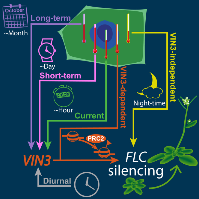
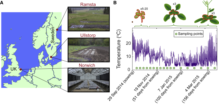
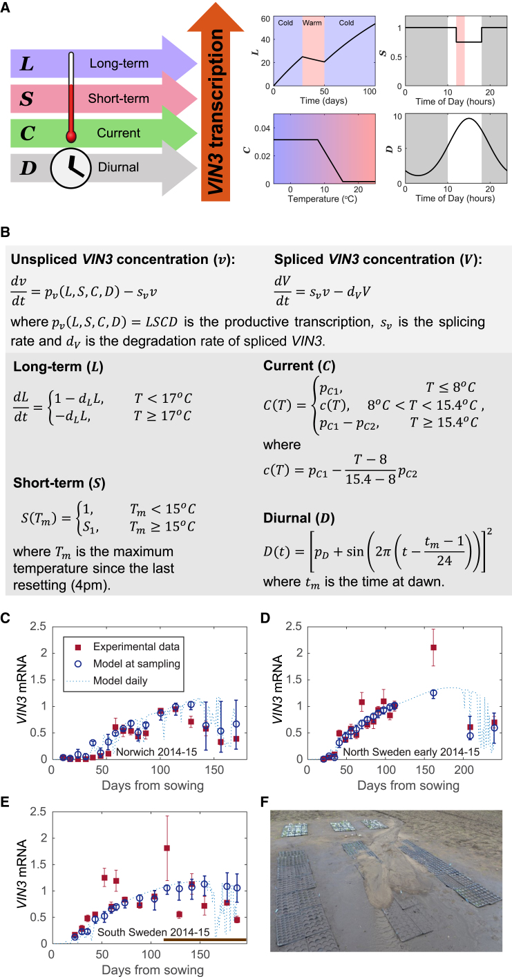
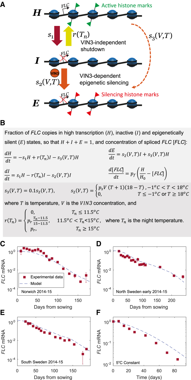
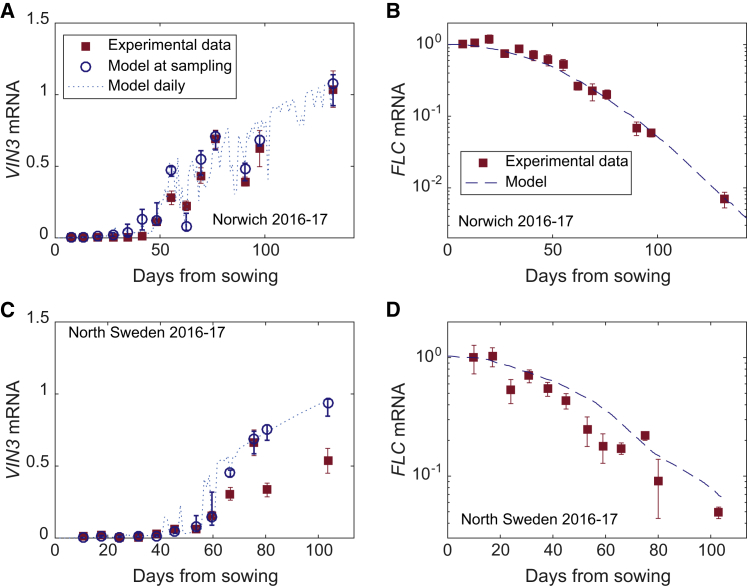
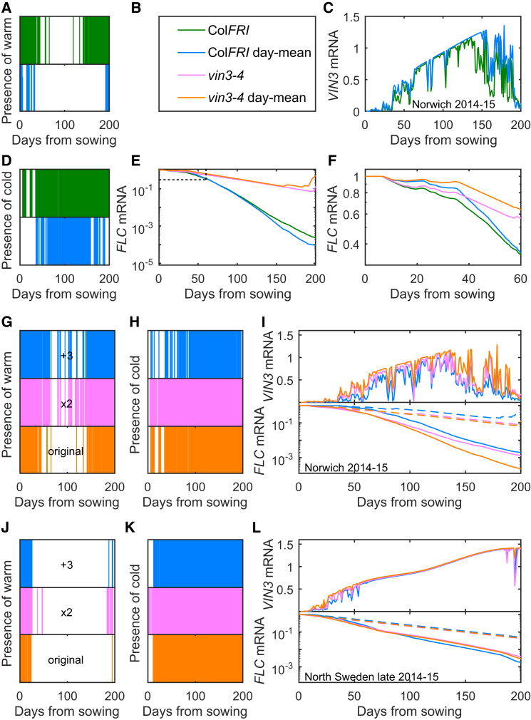
Many organisms need to respond to complex, noisy environmental signals for developmental decision making. Here, we dissect how Arabidopsis plants integrate widely fluctuating field temperatures over month-long timescales to progressively upregulate VERNALIZATION INSENSITIVE3 (VIN3) and silence FLOWERING LOCUS C (FLC), aligning flowering with spring. We develop a mathematical model for vernalization that operates on multiple timescales-long term (month), short term (day), and current (hour)-and is constrained by experimental data. Our analysis demonstrates that temperature sensing is not localized to specific nodes within the FLC network. Instead, temperature sensing is broadly distributed, with each thermosensory process responding to specific features of the plants' history of exposure to warm and cold. The model accurately predicts FLC silencing in new field data, allowing us to forecast FLC expression in changing climates. We suggest that distributed thermosensing may be a general property of thermoresponsive regulatory networks in complex natural environments.

Keywords: FLC; FLOWERING LOCUS C; VERNALIZATION INSENSITIVE3; VIN3; climate change; epigenetics; gene regulation; mathematical modeling; phenology; temperature sensing; vernalization.


Figures

None
Graphical abstract
Figure 1
Figure 1
Experimental Method for Field Experiments (A) Field sites in North Sweden (Ramsta), South Sweden (Ullstorp), and UK (Norwich). At the Swedish sites, plants were grown in trays bedded in the soil in the field. In Norwich, the plants were grown inside an unlit, unheated greenhouse with air-inlets, in trays bedded in vermiculite, ensuring the containment of transgenic lines while the plants still experienced natural conditions. (B) Example of sowing and sampling setup in the field experiments, showing the Norwich site 2014–2015. The temperature profile is shown together with the dates of sampling. Above the temperature plot, the approximate plant size throughout the experiment is shown, together with the tissues that were collected in the samples depending on the plants’ size (outlined in red), and the number of plants collected for each replicate. In Norwich, when plants were larger, only the youngest tissues were harvested, as indicated. 6 replicate samples were taken per time point, though some were lost in processing or unusable due to environmental factors, e.g., mudslides. See also Table S6.
Figure 2
Figure 2
Short Duration Spikes to High Temperature Affect VIN3 Expression (A) Temperature conditions given daily for 4 weeks (left) and then on day of sampling (right). Plants were grown in 20°C (night) or 22°C (day) 16-hr photoperiod for 1 week and then transferred to the conditions shown on the left. Dark background indicates nighttime (8-hr photoperiod). (B) VIN3 spliced expression during the day of sampling, sampled every 3 hr over a 12-hr period as shown. The green background indicates the time of the high temperature spike in the midday spike conditions. n = 1–9; average > 6. (C) VIN3 unspliced expression from experiment in (B). n = 1–9; average > 6. (D) VIN3 expression after 4 weeks cold in indicated conditions. “Before” refers to samples taken at 18:30 on sampling day, in the conditions indicated. “After” refers to samples that after 4 weeks cold in indicated conditions were further treated with, first, a further 4 days in the conditions indicated and then transferred in the afternoon (before dark) to constant 8°C conditions for approximately 24 hr before sampling at 18:30. n = 2–8; average = 4.4. (E) FLC expression averaged over all the time points of sampling day after 4 weeks cold. Kruskal-Wallis with Dunn’s post hoc test between midday spike, night spike and spike memory (conditions with similar VIN3 expression for the 4 weeks of the treatment to test for VIN3-independent effect only) gives p<0.05 significant difference ( in plot) between night spike and midday spike and between night spike and spike memory (no significant difference between midday spike and spike memory). Boxplots show median and 25th and 75th percentiles of the samples. Ends of whiskers show maximum and minimum values. n = 12–38; average > 30. In all cases, circle and bars show mean and standard error, respectively. RNA levels normalized to UBC, PP2A. See also Figures S3 and S4.
Figure 3
Figure 3
Description and Fitting of LSCD Model for VIN3 Dynamics (A) Diagram of the LSCD model showing the primary signals registered by each component, their temperature dependence, and how they affect VIN3 transcription. Element L increases slowly in the cold (<17°C) and decreases slowly in the warm. Element S remembers the presence of a high temperature spike until the evening and, during that time, remains decreased. Element C is high at low temperatures and low at high temperatures, changing linearly with temperature between 8°C and 15.4°C. Element D cycles each day, peaking in the afternoon. (B) Mathematical description of LSCD model showing the temperature and time dependency of each component. (C) Comparison of LSCD model and fitted experimental VIN3 mRNA data for Norwich in 2014–2015. Data from Hepworth et al. (2018), bars show mean and standard error, respectively. Model at sampling shows the mean of the predicted values of VIN3 mRNA in the sampling time window, which is defined as the period from 2 hr before the recorded sampling time to 2 hr after due to the long duration of sampling. The error bars show the maximum and minimum values of VIN3 mRNA during that time window. Model daily shows the predicted value for VIN3 mRNA at the same time every day (chosen as the time of the final sampling) to demonstrate the changes in amplitude of the VIN3 daily peak. (D) Comparison of model and experimental data from North Sweden (early planting) in 2014–2015, as described for Norwich in (C). (E) Comparison of model and experimental data from South Sweden in 2014–2015, as described for Norwich in (C). The late time points of the South Swedish data (brown bar) could not be fitted by our model, likely due to a mudslide (time given by start of brown bar) that damaged the plants and affected their VIN3 expression. (F) Mudslide at the South Swedish site covered the plants and caused sample losses. See also Figures S1–S3 and S5–S7.
Figure 4
Figure 4
Description and Fitting of Model for FLC Dynamics (A) Diagram of the FLC model showing switching between digital states in the FLC silencing pathway during vernalization. (B) Mathematical description of FLC model showing the temperature dependency of the switches. (C) Comparison of FLC model and fitted experimental FLC mRNA data for Norwich, in 2014–2015 (data from Hepworth et al. [2018]). (D) Comparison of FLC model and experimental data for North Sweden (early planting) in 2014–15 (data from Hepworth et al. [2018]). (E) Comparison of FLC model and experimental data for South Sweden in 2014–15 (data from Hepworth et al. [2018]). (F) Comparison of FLC model and fitted experimental FLC mRNA data for Constant 5°C (combined data from Figure S9B). In all cases, squares and bars show mean and standard error, respectively. See also Figures S5, S6, S8, and S9.
Figure 5
Figure 5
Validation of VIN3/FLC Model (A and B) Validation of VIN3/FLC model by prediction of (A) VIN3 and (B) FLC behavior under new field conditions in Norwich 2016–2017. n = 4–6; average > 5.4. (C and D) As for (A) and (B) for new field conditions in North Sweden 2016–2017. n = 3–6; average > 4.6. For data, squares and bars show mean and standard error, respectively, while for the model, circles show the mean of the predicted values of VIN3 mRNA in the sampling time window and bars show the maximum and minimum values during that time window. See also Figures S6 and S10.
Figure 6
Figure 6
Assessment of Climate Sensitivity of FLC and VIN3 Dynamics (A–F) Norwich 2014–2015 prediction for ColFRISf2 (ColFRI, green) compared to the prediction where the temperature at each time point is replaced by the 24-hr average temperature of that day (ColFRI day-mean, blue). The same is shown also for the vin3-4 mutant (pink and orange, respectively). (A) shows “presence of warm” features in the two temperature profiles, green for measured temperature, and blue for day-mean temperature. Presence of color stripe corresponds to a high temperature spike on that day (day maximum above 15°C). (B) Figure legend for (A)–(F). (C) VIN3 mRNA prediction, for ColFRI. (D) shows “presence of cold” features in the two temperature profiles, green for measured temperature and blue for day-mean temperature. Presence of color stripe corresponds to a low temperature dip on that day (day minimum below 10°C). (E and F) FLC mRNA prediction, for ColFRI and vin3-4 mutant. (F) shows the same predictions as (E) but only for the first 60 days, as indicated by dashed line square in (E). (G) “Presence of warm” features in three temperature profiles, Norwich 2014–2015 (orange), the Norwich profile modified by adding 3°C (“+3,” blue) or by stretching the temperatures around the daily mean (“x2,” pink). (H) “Presence of cold” features in the modified temperature profiles as described in (G). (I) FLC and VIN3 mRNA predictions based on Norwich 2014–2015 temperature (orange) compared to the modified profiles as in (G) and (H). Dashed lines are for vin3-4 mutant. (J) “Presence of warm” features in three temperature profiles, North Sweden 2014–2015 (orange), the North Sweden profile modified by adding 3°C (“+3,” blue) or by stretching the temperatures around the daily mean (“x2,” pink). (K) “Presence of cold” features in the modified temperature profiles as described in (J). (L) FLC and VIN3 mRNA predictions based on North Sweden 2014–2015 temperature (orange) compared to the modified profiles as in (J) and (K). Dashed lines are for vin3-4 mutant. In all cases, temperatures are from Hepworth et al., (2018). See also Figure S11.

References

    1. Aikawa S., Kobayashi M.J., Satake A., Shimizu K.K., Kudoh H. Robust control of the seasonal expression of the Arabidopsis FLC gene in a fluctuating environment. Proc. Natl. Acad. Sci. USA. 2010;107:11632–11637. - PMC - PubMed
    1. Andrés F., Coupland G. The genetic basis of flowering responses to seasonal cues. Nat. Rev. Genet. 2012;13:627–639. - PubMed
    1. Angel A., Song J., Dean C., Howard M. A Polycomb-based switch underlying quantitative epigenetic memory. Nature. 2011;476:105–108. - PubMed
    1. Angel A., Song J., Yang H., Questa J.I., Dean C., Howard M. Vernalizing cold is registered digitally at FLC. Proc. Natl. Acad. Sci. USA. 2015;112:4146–4151. - PMC - PubMed
    1. Berry S., Hartley M., Olsson T.S.G., Dean C., Howard M. Local chromatin environment of a Polycomb target gene instructs its own epigenetic inheritance. Elife. 2015;4:e07205. - PMC - PubMed

Publication types

LinkOut - more resources