A stochastic framework to model axon interactions within growing neuronal populations

Abstract

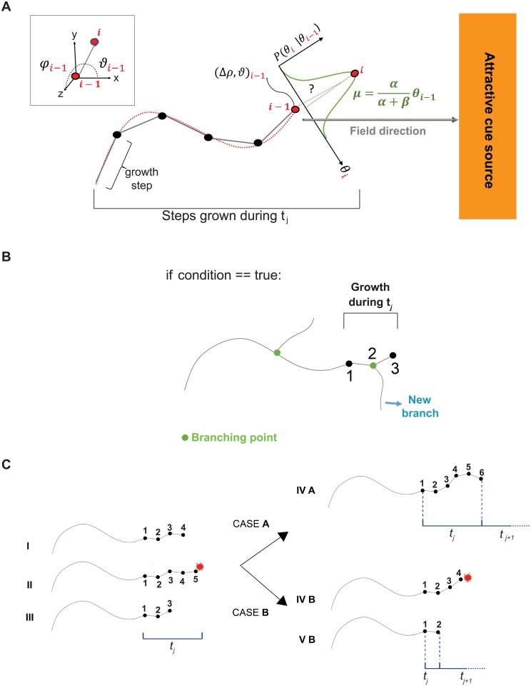
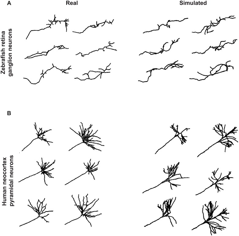
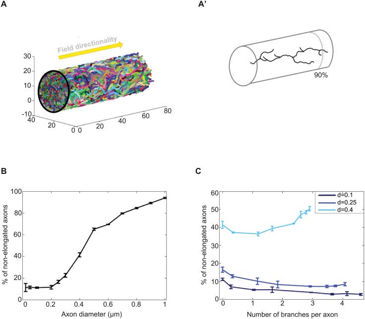
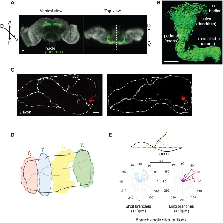
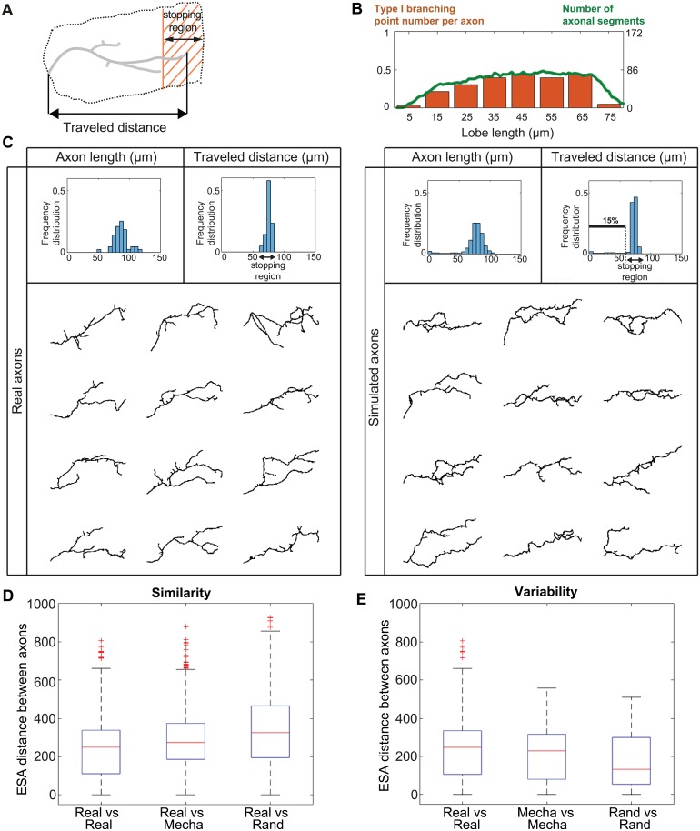
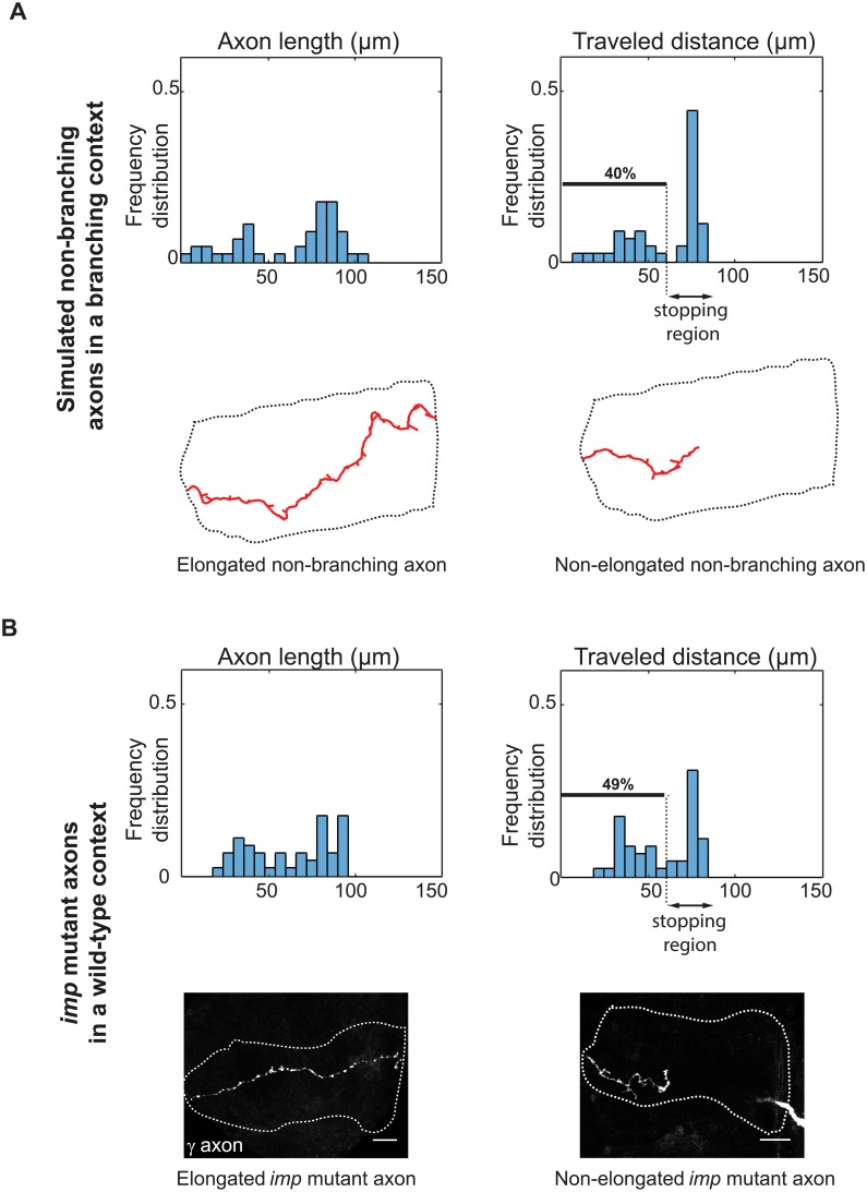
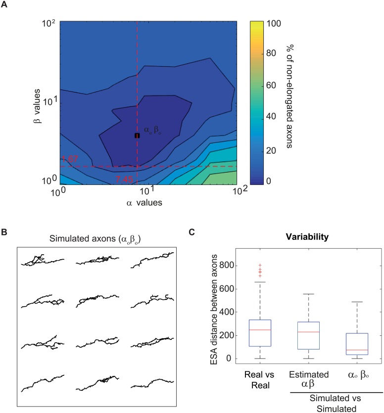
The confined and crowded environment of developing brains imposes spatial constraints on neuronal cells that have evolved individual and collective strategies to optimize their growth. These include organizing neurons into populations extending their axons to common target territories. How individual axons interact with each other within such populations to optimize innervation is currently unclear and difficult to analyze experimentally in vivo. Here, we developed a stochastic model of 3D axon growth that takes into account spatial environmental constraints, physical interactions between neighboring axons, and branch formation. This general, predictive and robust model, when fed with parameters estimated on real neurons from the Drosophila brain, enabled the study of the mechanistic principles underlying the growth of axonal populations. First, it provided a novel explanation for the diversity of growth and branching patterns observed in vivo within populations of genetically identical neurons. Second, it uncovered that axon branching could be a strategy optimizing the overall growth of axons competing with others in contexts of high axonal density. The flexibility of this framework will make it possible to investigate the rules underlying axon growth and regeneration in the context of various neuronal populations.

Fig 1. 3D mathematical model of individual axon growth.

(A) The axon elongates step by step (grey segments), each step being delimited by the current point in space i and the previous one, i − 1. Each i^th new step is described by its spherical coordinates (Δρ, ϑ, φ) (represented in 2D for simplicity; see upper left corner for a 3D view), and placed after the previous position i − 1. The exact position of the i^th point is defined (in 2D) by ${\theta }_{xy}^i=f\left({\varphi }_{x,y}^i\right)$, which is drawn from a conditional Normal probability distribution (in green). The most probable value (mean of the distribution (μ)) considers the directions of the last step i − 1 and of the attractive field, each contribution weighted by α and β respectively. For each time unit t_j, a maximum number of steps (n_max) is allowed. (B) Algorithmic implementation of branch generation. During t_j, a certain number of growth steps are performed (3 in this schematic representation). At the end of t_j, a certain “condition” is evaluated and, if true, a branch point is placed at the axon tip, or at any other step performed during t_j (step 2). (C) Step by step axon growth scheme during t_j considering physical interactions. The axon elongates of n steps (I), until it encounters a mechanical constraint (II) and retracts (III). During the same time interval t_j, it will re-try to reach n_max steps (6 in this example). If no other mechanical constraint is encountered (CASE A), the axon will advance to reach n_max steps. If, on the contrary, another mechanical constraint is encountered (CASE B), the axon will retract again and stop its growth until the next time point (t_j+1). In this case, the total growth during t_j is then smaller than n_max steps.

Fig 2. Examples of axonal morphologies generated by the model and comparison to real data.

(A) Real (left) and simulated (right) axonal trees of zebrafish retina ganglion neurons. (B) Real (left) and simulated (right) axonal trees of human neocortex pyramidal neurons. Real axonal trees were obtained from the Neuromorpho.org database. Simulated axons where generated in isolation, using the following parameter values (Zebrafish/Human): for the main axon α = 15/10 and β = 2/30; for the branches α = 20/100 and β = 0.5/10, Δρ = 1/3, ψ = 0 rad ∀x / 0 rad. for x ≤ 60 μm, +(−)1.3 rad for x > 60 μm and y > 0(y ≤ 0), P_b = 0.5/0 for x < 60 μm and 0.3 otherwise, ω: uniform in all the space/ uniform in a solid angle of $\frac{\pi }{4}$ respect to the neurite from which the branch emerges, λ_b = 6/1, b_l = 2/2, n_max = 10/1, X_max = 80/110. In addition, for the human neocortex pyramidal neurons, branch maximum lengths follow a normal distribution of mean 100 μm and standard deviation 70 μm.

Fig 3. Simulations of axons growing collectively in a confined environment.

(A) 400 axons were simulated growing inside a cylinder of fixed diameter and length. Left: whole population. Right: example of an individual properly-elongated axon generated with d = 0.4 μm and P_b = 0.5. Axons were defined as properly elongated if at least one of their branch tip reached 90% of the cylinder length. The external field (ψ) directionality is represented as an arrow. (B) Percentage of non-elongated axons in function of the axon diameter value. (C) Percentage of non-elongated axons in function of branch number for different axonal diameter values. The error bars in B and C represent the standard deviation observed after running 3 simulations. The following parameter values were used: α = 9 and β = 2, Δρ = 1, ψ = 0 rad, ω: uniform in all the space, λ_b = 15, b_l = 1, d: indicated in each case, Num_ax = 400, n_max = 6, n_r = 2, counter_max = 140, X_max = 70 and ξ: tube of radius 13 μm. P_b = 0 was used in B and for the “no branch” condition in C. Increasing values of P_b were used to increase the number of branches per axon (S2B Fig).

Fig 4. Characteristics of adult Mushroom Body γ neurons.

(A) Wild-type adult Drosophila brain expressing the membrane-tagged CD8-GFP construct in γ neurons, under the control of the MB009B-Gal4. Nuclei are labeled in white with DAPI. The dotted line on the top view image corresponds to the midline. (B) 3D reconstruction of one Mushroom Body where γ neurons only were labeled. Genotype: MB009B-Gal4/UAS CD8-GFP. (C) Axonal arborizations of two individual adult γ neurons labeled by GFP using the MARCM technique. Confocal images taken along the z axis were projected (Maximum Intensity Projection). Dotted lines delimit the shape of the medial lobe. Red arrows indicate axon tips that reached the extremity of the medial lobe. (D) Schematic representation of the different anatomical domains (distinguished with different colors) defined along the medial lobe and innervated by distinct input and output neurons. Adapted from [34]. Scale bars: 20 μm in A, 50 μm in B and 10 μm in C. (E) Top panel: schematic representation of how directionality angles were measured. We have considered the angle between the vector defined by the first and last point of the mother branch (red segment), and the vector defined by the first and last point of the considered branch (yellow segment) projected on the xy plane. Bottom panel: frequency distribution of the directionality angles of long (>10 μm, type I) and short (<10 μm, type II) branches measured on reconstructed wild-type adult γ axons. The frequency values are presented as a percentage of each group (n = 97 and 283 for type I and II branches respectively). The middle circle represents 10 and 15% for type II and I respectively. *** stands for p = 4.4⁻¹³ (Kruskal Wallis test).

Fig 5. Simulation of γ axon growth within a population of interacting axons.

(A) Schematic representation of a single main γ axon within the medial lobe. Both the stopping region (shaded region) and the traveled distance (projection along the horizontal axis) are indicated. Axonal trees that fail to elongate a branch reaching the stopping region are considered as non-elongated. (B) Correlation between the spatial distribution of type I branching point number and axonal density. The orange bars represent the number of type I branching points per axon along the lobe axis. The green curve represents the number of axonal segments found in each lobe region. Data from reconstructed real axons were used for this analysis. (C) Top: Frequency distributions of 2D-projected main axon lengths (left panels), and traveled distances within the medial lobe (right panels). Data from real wild-type γ axons are shown in the left panels (n = 43), and data from simulated ones in the right panels (n = 650). The black arrows indicate the stopping region. The distributions of 3D main axon lengths are shown in S8A Fig. The definition of main axon is provided in Supporting information. Bottom: Examples of reconstructed real single wild-type γ axons (left) and simulated γ axons (right). (D) Measure of similarity between real and simulated axons. Boxplots of inter-axon distances within the population of real axons (real, n = 43), and between real and simulated axons, considering either mechanical (mecha) or random (rand) branching (n = 50 in both cases). (E) Measure of intra-population morphological variability. Boxplots of inter-axon distances within the population of real axons (real, n = 43), and within the population of simulated axons, considering either mechanical or random branching (n = 50 in both cases). Inter-axon distances were calculated with the ESA distance [40]. Boxplots were created following the original plotting convention of Tukey. The central mark indicates the median, the bottom and top edges of the box indicate the 25^th and 75^th percentiles, respectively. The whiskers extend to the most extreme data points not considered as outliers. Outliers are plotted individually using the ‘+’ symbol.

Fig 6. Out-competition of non-branching axons by branching ones.

(A) Top: frequency distributions of 2D-projected axon lengths and traveled distances of single simulated non-branching axons grown in the context of otherwise branching axons. 40% of axons fail to reach the lobe extremity in this condition (n = 45). Bottom: examples of fully elongated (left) and growth-defective (right) simulated single axons. (B) Top: frequency distributions of axon lengths and traveled distances of single imp⁷ mutant axons grown in the context of a wild-type population. A bimodal behavior similar to that generated by simulations is observed (n = 45). Lower panels: example of fully elongated (left) and growth-defective (right) imp⁷ single axons grown in a wild-type environment and labeled with GFP. Scale bar 10 μm.

Fig 7. Impact of α and β values on axon morphologies.

(A) Percentage of axons failing to reach the lobe extremity in function of pairs of parameter values. The dotted lines correspond to the parameter values estimated from data (see Parameter Estimation). The square shows the pair of parameter values minimizing the percentage of axons that do not reach the lobe extremity (α_o and β_o). (B) Examples of γ axon morphologies from simulations with the parameters that optimize axon growth at the population level (α_o β_o). (C) Boxplots of inter-axon distances within the population of real axons (real, n = 43), axons simulated with the estimated parameters (estimated α β, n = 50), and axons simulated with the α_o β_o parameters (n = 50). Inter-axon distances were calculated with the ESA distance [40]. Boxplots were created following the original plotting convention of Tukey. The central mark indicates the median, the bottom and top edges of the box indicate the 25^th and 75^th percentiles, respectively. The whiskers extend to the most extreme data points not considered as outliers. Outliers are plotted individually using the ‘+’ symbol.

References

1. Bixby JL, Harris WA. Molecular mechanisms of axon growth and guidance. Annual Review of Cell Biology. 1991;7:117–59. 10.1146/annurev.cb.07.110191.001001 - DOI - PubMed
1. Tessier-Lavigne M, Goodman CS, et al. The molecular biology of axon guidance. Science. 1996;274(5290):1123–1133. 10.1126/science.274.5290.1123 - DOI - PubMed
1. Song Hj, Poo Mm. The cell biology of neuronal navigation. Nature cell biology. 2001;3(3):E81–E88. 10.1038/35060164 - DOI - PubMed
1. Dickson BJ. Molecular mechanisms of axon guidance. Science. 2002;298(5600):1959–1964. 10.1126/science.1072165 - DOI - PubMed
1. Guan KL, Rao Y. Signalling mechanisms mediating neuronal responses to guidance cues. Nature Reviews Neuroscience. 2003;4(12):941–956. 10.1038/nrn1254 - DOI - PubMed
Publication types
MeSH terms
LinkOut - more resources