. 2018 Dec 3;16(12):e2005127.
doi: 10.1371/journal.pbio.2005127. eCollection 2018 Dec.

Neural responses to natural and model-matched stimuli reveal distinct computations in primary and nonprimary auditory cortex

Affiliations

Neural responses to natural and model-matched stimuli reveal distinct computations in primary and nonprimary auditory cortex

Sam V Norman-Haignere et al. PLoS Biol. .

Abstract

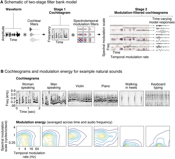
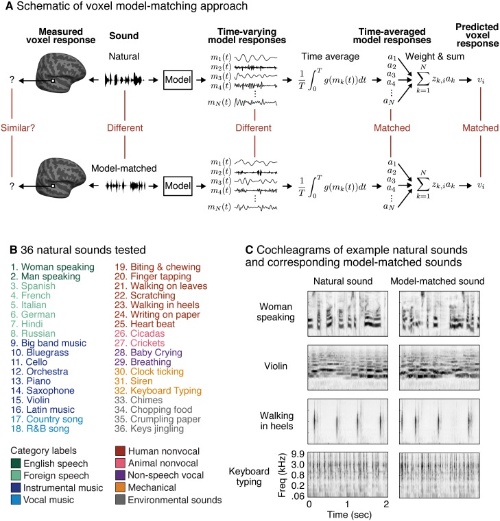
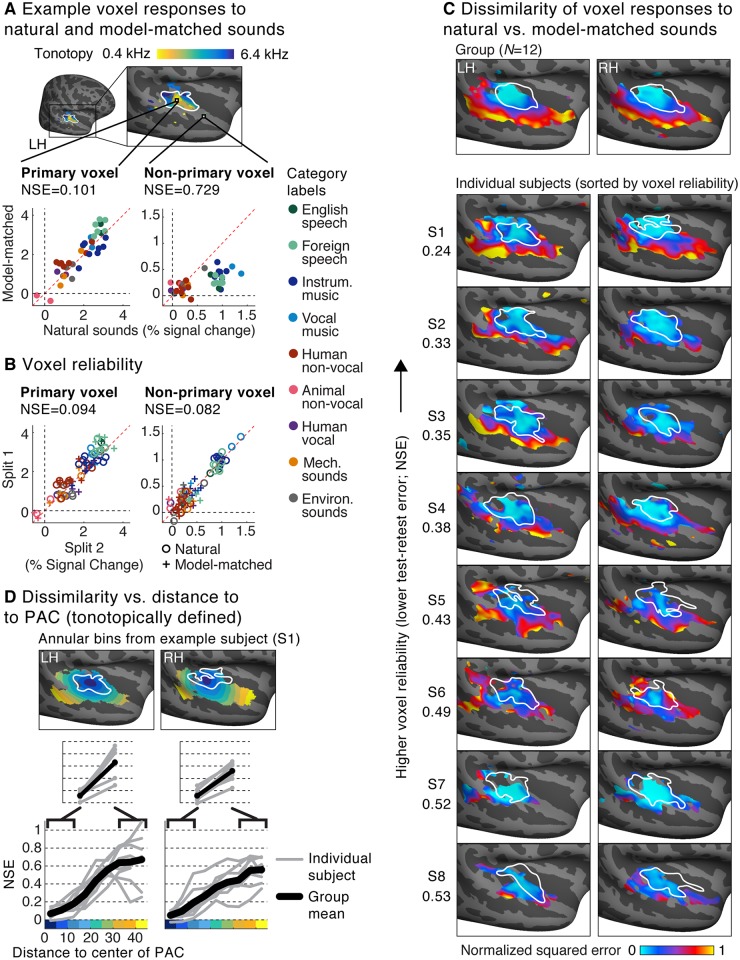
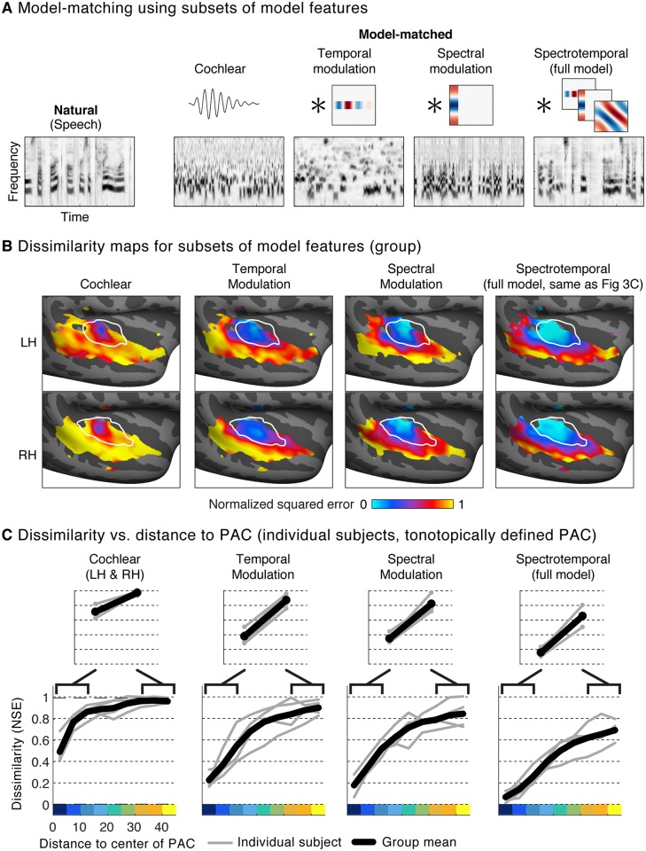
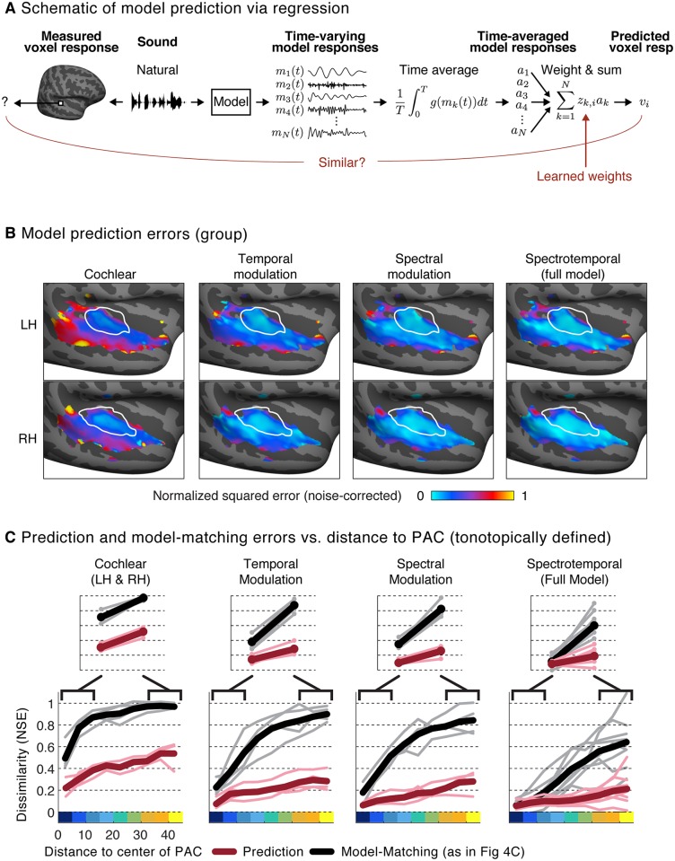
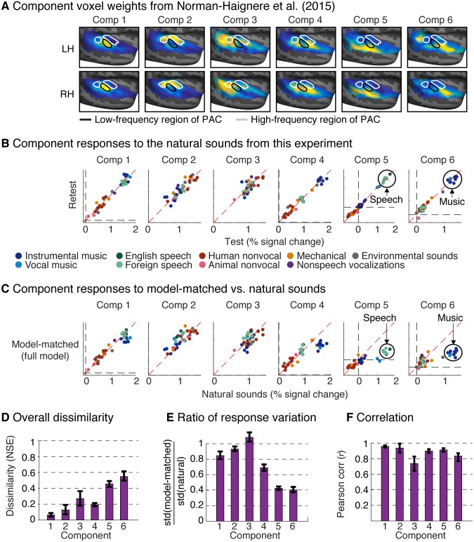
A central goal of sensory neuroscience is to construct models that can explain neural responses to natural stimuli. As a consequence, sensory models are often tested by comparing neural responses to natural stimuli with model responses to those stimuli. One challenge is that distinct model features are often correlated across natural stimuli, and thus model features can predict neural responses even if they do not in fact drive them. Here, we propose a simple alternative for testing a sensory model: we synthesize a stimulus that yields the same model response as each of a set of natural stimuli, and test whether the natural and "model-matched" stimuli elicit the same neural responses. We used this approach to test whether a common model of auditory cortex-in which spectrogram-like peripheral input is processed by linear spectrotemporal filters-can explain fMRI responses in humans to natural sounds. Prior studies have that shown that this model has good predictive power throughout auditory cortex, but this finding could reflect feature correlations in natural stimuli. We observed that fMRI responses to natural and model-matched stimuli were nearly equivalent in primary auditory cortex (PAC) but that nonprimary regions, including those selective for music or speech, showed highly divergent responses to the two sound sets. This dissociation between primary and nonprimary regions was less clear from model predictions due to the influence of feature correlations across natural stimuli. Our results provide a signature of hierarchical organization in human auditory cortex, and suggest that nonprimary regions compute higher-order stimulus properties that are not well captured by traditional models. Our methodology enables stronger tests of sensory models and could be broadly applied in other domains.


Conflict of interest statement

The authors have declared that no competing interests exist.

Figures

Fig 1
Fig 1. Illustration of the auditory model tested in this study.
(A) The model consists of two cascaded stages of filtering. In the first stage, a cochleagram is computed by convolving each sound with audio filters tuned to different frequencies, extracting the temporal envelope of the resulting filter responses, and applying a compressive nonlinearity to simulate the effect of cochlear amplification (for simplicity, envelope extraction and compression are not illustrated in the figure). The result is a spectrogram-like structure that represents sound energy as a function of time and frequency. In the second stage, the cochleagram is convolved in time and frequency with filters that are tuned to different rates of temporal and spectral modulation. The output of the second stage can be conceptualized as a set of filtered cochleagrams, each highlighting modulations at a particular temporal rate and spectral scale. Each frequency channel of these filtered cochleagrams represents the time-varying output of a single model feature that is tuned to audio frequency, temporal modulation rate, and spectral modulation scale. (B) Cochleagrams and modulation spectra are shown for six example natural sounds. Modulation spectra plot the energy (variance) of the second-stage filter responses as a function of temporal modulation rate and spectral modulation scale, averaged across time and audio frequency. Different classes of sounds have characteristic modulation spectra.
Fig 2
Fig 2. Model-matching methodology and experimental stimuli.
(A) The logic of the model-matching procedure, as applied to fMRI. The models we consider are defined by the time-varying response of a set of model features (mk(t)) to a sound (as in the auditory model shown in Fig 1A). Because fMRI is thought to pool activity across neurons and time, we modeled fMRI voxel responses as weighted sums of time-averaged model responses (Eqs 1 and 2, with ak corresponding to the time-averaged model responses and zk,i to the weight of model feature k in voxel i). Model-matched sounds were designed to produce the same time-averaged response for all of the features in the model (all ak matched) and thus to yield the same voxel response (for voxels containing neurons that can be approximated by the model features), regardless of how these time-averaged activities are weighted. The temporal response pattern of the model features was otherwise unconstrained. As a consequence, the model-matched sounds were distinct from the natural sounds to which they were matched. (B) Stimuli were derived from a set of 36 natural sounds. The sounds were selected to produce high response variance in auditory cortical voxels, based on the results of a prior study [45]. Font color denotes membership in one of nine semantic categories (as determined by human listeners [45]). (C) Cochleagrams are shown for four natural and model-matched sounds constrained by the spectrotemporal modulation model shown in Fig 1A.
Fig 3
Fig 3. Voxel responses to natural and model-matched sounds.
(A) Responses to natural and model-matched sounds from two example voxels from a single subject. One voxel is drawn from the low-frequency region of PAC (defined tonotopically) and one from outside of PAC. A tonotopic map measured in the same subject is shown for anatomical comparison; the map plots the pure tone frequency that produced the highest voxel response. Each dot represents the response to a single pair of natural and model-matched sounds. The primary voxel responded similarly to natural and model-matched sounds, while the nonprimary voxel exhibited a weaker response to model-matched sounds. We quantified the dissimilarity of voxel responses to natural and model-matched sounds using a normalized squared error metric (NSE) metric (see text for details). (B) Split-half reliability of the responses to natural (circles) and model-matched sounds (crosses) for the two voxels shown in panel A. Both primary and nonprimary voxels exhibited a reliable response (and thus a low NSE between the two measurements). (C) Maps plotting the NSE between each voxel’s response to natural and model-matched sounds, corrected for noise in fMRI measurements (see S4 Fig for uncorrected maps). Maps are shown both for voxel responses from eight individual subjects (who were scanned more than the other subjects) and for group responses averaged across 12 subjects in standardized anatomical coordinates (top). The white outline plots the boundaries of PAC, defined tonotopically. Only voxels with a reliable response were included (see text for details). Subjects are sorted by the median test-retest reliability of their voxel responses in auditory cortex, as measured by the NSE (the number to the left of the maps for each subject). (D) A summary figure plotting the dissimilarity of voxel responses to natural and model-matched sounds as a function of distance to the low-frequency region of PAC (see S5 Fig for an anatomically based analysis). This figure was computed from the individual subject maps shown in panel C. Voxels were binned based on their distance to PAC in 5-mm intervals. The bins for one example subject (S1) are plotted. Each gray line represents a single subject (for each bin, the median NSE value across voxels is plotted), and the black line represents the average across subjects. Primary and nonprimary auditory cortex were defined as the average NSE value across the three bins closest and farthest from PAC (inset). In every subject and hemisphere, we observed larger NSE values in nonprimary regions. Note that the left hemisphere has been flipped in all panels to facilitate comparison between the left and right hemispheres. LH, left hemisphere; PAC, primary auditory cortex; RH, right hemisphere.
Fig 4
Fig 4. Comparison of responses to model-matched sounds constrained by different models.
(A) Cochleagrams for an example natural sound and several corresponding model-matched sounds constrained by subsets of features from the full two-stage model. Cochlear-matched sounds were constrained by time-averaged statistics of the cochleagram representation but not by any responses from the second-stage filters. As a consequence, they had a similar spectrum and overall depth of modulation as the corresponding natural sound, but were otherwise unconstrained. The other three sounds were additionally constrained by the response of second-stage filters, tuned either to temporal modulation, spectral modulation, or both temporal and spectral modulation (the full model used in Fig 3). Temporal modulation filters were convolved separately in time with each cochlear frequency channel. Spectral modulation filters were convolved in frequency with each time slice of the cochleagram. In this example, the absence of spectral modulation filters causes the frequency channels to become less correlated, while the absence of temporal modulation filters results in a signal with more rapid temporal variations than that present in natural speech. (B) Maps of the NSE between responses to natural and model-matched sounds, constrained by each of the four models. The format is the same as panel 3C. See S7 Fig for maps from individual subjects. (C) Dissimilarity between responses to natural and model-matched sounds versus distance to the low-frequency area of PAC. Format is the same as panel 3D. Results are based on data from the four subjects that participated in Paradigm I, because model-matched sounds constrained by subsets of features were not tested in Paradigm II. LH, left hemisphere; NSE, normalized squared error; PAC, primary auditory cortex; RH, right hemisphere.
Fig 5
Fig 5. Predicted responses to natural sounds via regression using the same auditory model used to constrain the model-matched sounds.
(A) Schematic of regression procedure used to predict neural responses from model features. For each natural sound, we computed the response time course for each feature in the model, as was done for model matching. We then computed a time-averaged measure of each feature’s activity (the mean across time for the cochlear features, because they are the result of an envelope operation, and the standard deviation for the modulation features, because they are raw filter outputs) and estimated the weighted combination of these time-averaged statistics that yielded the best-predicted response (using ridge regression, cross-validated across sounds). (B) Maps showing the prediction error (using the same NSE metric employed in Figs 3 and 4) between measured and predicted responses to natural sounds for the corresponding models shown in Fig 4 (see S8 Fig for maps from individual subjects). (C) Prediction error versus distance to the low-frequency area of PAC (maroon lines: thin lines correspond to individual subjects, thick lines correspond to the group average). For comparison, the corresponding NSE values derived from the model-matching procedure are replotted from Fig 4C (black lines). The analyses are based on individual subject maps. Results for the full model (rightmost plot) are based on data from the same eight subjects shown in Fig 3C. Results for model subsets (cochlear, temporal modulation, and spectral modulation) are based on data from four subjects that were scanned in Paradigm I (sounds constrained by subsets of model features were not tested in Paradigm II). LH, left hemisphere; NSE, normalized squared error; PAC, primary auditory cortex; RH, right hemisphere.
Fig 6
Fig 6. Voxel decomposition of responses to natural and model-matched sounds.
Previously, we found that much of the voxel response variance to natural sounds can be approximated as a weighted sum of six canonical response patterns (“components”) [45]. This figure shows the response of these components to the natural and model-matched sounds from this experiment. (A) The group component weights from Norman-Haignere and colleagues (2015) [45] are replotted to show where in auditory cortex each component explains the neural response. (B) Test-retest reliability of component responses to the natural sounds from this study. Each data point represents responses to a single sound, with color denoting its semantic category. Components 5 and 6 showed selectivity for speech and music, respectively, as expected (Component 4 also responded most to music because of its selectivity for sounds with pitch). (C) Component responses to natural and model-matched sounds constrained by the complete spectrotemporal model (see S11 Fig for results using subsets of model features). The speech and music-selective components show a weak response to model-matched sounds, even for sounds constrained by the full model. (D) NSE between responses to natural and model-matched sounds for each component. (E) The ratio of the standard deviation of each component’s responses to model-matched and natural sounds (see S12A Fig for corresponding whole-brain maps). (F) Pearson correlation of responses to natural and model-matched sounds (see S12B Fig for corresponding whole-brain maps). All of the metrics in panels D—F are noise-corrected, although the effect of this correction is modest because the component responses are reliable (as is evident in panel B). Error bars correspond to one standard error computed via bootstrapping across subjects. LH, left hemisphere; NSE, normalized squared error; PAC, primary auditory cortex; RH, right hemisphere.

Similar articles

Cited by

References

    1. Simoncelli EP, Olshausen BA. Natural image statistics and neural representation. Annu Rev Neurosci. 2001;24: 1193–1216. 10.1146/annurev.neuro.24.1.1193 - DOI - PubMed
    1. Woolley SM, Fremouw TE, Hsu A, Theunissen FE. Tuning for spectro-temporal modulations as a mechanism for auditory discrimination of natural sounds. Nat Neurosci. 2005;8: 1371–1379. 10.1038/nn1536 - DOI - PubMed
    1. Smith EC, Lewicki MS. Efficient auditory coding. Nature. 2006;439: 978–982. 10.1038/nature04485 - DOI - PubMed
    1. Sharpee T, Rust NC, Bialek W. Analyzing neural responses to natural signals: maximally informative dimensions. Neural Comput. 2004;16: 223–250. 10.1162/089976604322742010 - DOI - PubMed
    1. Naselaris T, Kay KN, Nishimoto S, Gallant JL. Encoding and decoding in fMRI. Neuroimage. 2011;56: 400–410. 10.1016/j.neuroimage.2010.07.073 - DOI - PMC - PubMed

Publication types