Review
. 2018 Dec 2;62(5):643-723.
doi: 10.1042/EBC20170053. Print 2018 Dec 3.

The genetic basis of disease

Affiliations
Review

The genetic basis of disease

Maria Jackson et al. Essays Biochem. .

Erratum in

  • Correction: The genetic basis of disease.
    Jackson M, Marks L, May GHW, Wilson JB. Jackson M, et al. Essays Biochem. 2020 Oct 8;64(4):681. doi: 10.1042/EBC20170053_COR. Essays Biochem. 2020. PMID: 32720679 Free PMC article. No abstract available.

Abstract

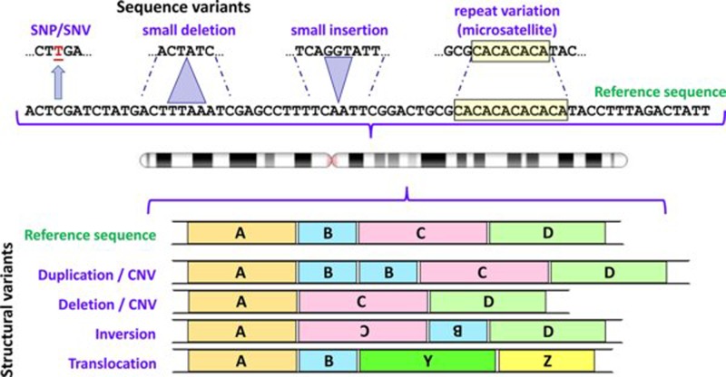
Genetics plays a role, to a greater or lesser extent, in all diseases. Variations in our DNA and differences in how that DNA functions (alone or in combinations), alongside the environment (which encompasses lifestyle), contribute to disease processes. This review explores the genetic basis of human disease, including single gene disorders, chromosomal imbalances, epigenetics, cancer and complex disorders, and considers how our understanding and technological advances can be applied to provision of appropriate diagnosis, management and therapy for patients.

Keywords: cancer; genetics; genomics; molecular basis of health and disease.


Conflict of interest statement

The authors declare that there are no competing interests associated with the manuscript.

Figures

Figure 1
Figure 1. Some types of variants found in human genomes
Variation involving one or a few nucleotides are shown above the chromosome icon, and structural variants below; in each case the variants are depicted in relation to the reference sequence. For depiction of structural variants A, B, C and D represent large segments of DNA; Y and Z represent segments of DNA from a different chromosome. Note that differentiation between CNVs and deletions/insertions depends upon the size of the relevant DNA segment (see text for further details). Abbreviation: CNV, copy number variant. Chromosome ideogram from NCBI Genome Decoration Page.
Figure 2
Figure 2. Giemsa banding (G-banding) to form a karyogram
(A) Metaphase spreads like this are obtained from cultured cells arrested in metaphase using colcemid, followed by Giemsa staining to create characteristic light and dark bands. Generally the dark bands represent regions which are AT-rich and gene-poor. (B) The chromosomes from the spread are arranged in pairs to view the karyotype, often using specialist software like Cytovision. (C) Diagrammatic representations of the G-banding patterns, called ideograms, are used as a reference. The ideograms have been aligned at the centromere (dotted line); blue shaded regions are highly variable – note for example the variation between p arms of chromosome 13, 14 and 15 in (B). In fact the p arms of the acrocentric chromosomes (13, 14, 15, 21, 22) all have very similar content, which includes the nucleolar organiser regions or NORs. Each NOR contains a tandem repeat of ribosomal DNA (rDNA) which encodes the rRNAs. Between all five acrocentrics there are approximately 300–400 rDNA repeats, though the actual number varies between individuals. Chromosome ideograms from NCBI Genome Decoration Page.
Figure 3
Figure 3. Chromosome structure and band nomenclature
This ideogram of the complete chromosome 8 illustrates the general structure of all human chromosomes: short (p) and long (q) arms, joined at the centromere. Each chromosome has a characteristic G-banding pattern, with each band annotated, for example p22 or q23. In chromosomes which are less condensed, more bands are seen as separate entities, while bands may merge together in more condensed chromosomes (for example, q21.1, q21.2 and q21.3 appear as a single band [q21] in a more condensed chromosome 8). The approved way of stating the location q21.1 is q-two-one-point-one (not q-twenty-one-point-one). Telomeres, with a shared structure, are present at both ends of each chromosome. Each telomere is composed of arrays of TTAGGG repeats, followed by a subtelomere, which is formed of repetitive sequences which can be similar between several telomeres. Chromosome ideogram from NCBI Genome Decoration Page.
Figure 4
Figure 4. Principles of meiosis and non-disjunction
For simplicity, only one pair of newly replicated autosomes is shown in two different colours to distinguish the maternal from the paternal chromosome and crossover is not considered. During spermatogenesis, all four meiotic products can form the gametes (sperm), while in oogenesis, only one of the four products will actually become the ovum (egg) as one daughter cell forms a polar body at meiosis I (MI) and another forms a polar body at meiosis II (MII). For clarity, all four potential meiotic products are shown. (A) During normal meiosis, four haploid meiotic products are formed. (B) If non-disjunction occurs during MI, two daughter cells are formed which completely lack this particular chromosome (nullisomic for this chromosome), while two others contain two copies of the chromosome (disomic). (C) If non-disjunction occurs during MII, one nullisomic and one disomic daughter cell is formed, while the remaining two form normally.
Figure 5
Figure 5. Fertilisation outcomes
(A) Fertilisation of a normal oocyte with a normal sperm cell leads to the formation of a diploid (2n) zygote. (B) If a nullisomic oocyte is fertilised, the resulting zygote will be monosomic for one chromosome. (C,D) Fertilisation of a disomic oocyte results in trisomic zygotes. Note that in (C), the oocyte has resulted from non-disjunction in meiosis I, and the resulting zygote contains one chromosome (ignoring crossover) from each maternal grandparent as well as the paternal contribution. In (D), the oocyte has resulted from non-disjunction in meiosis II, and the resulting zygote contains two chromosomes (aside from crossover regions) from one grandparent.
Figure 6
Figure 6. Segregation of reciprocal translocations
(A) A carrier of a reciprocal translocation has one unaltered copy of each chromosome that participates in the translocation, together with two hybrid chromosomes. Only the relevant chromosomes are shown, for illustration each is labelled with a circled number. (B) During meiosis, replicated sister chromatids pair up with their homologues. In the case of a translocation carrier, so-called ‘quadrivalents’ can form, in which four instead of two chromosomes pair up. (C) Three possible segregation paths are illustrated. During ‘alternate’ segregation, chromosomes 1 and 4, and chromosomes 2 and 3 are segregated into separate gametes. ‘Adjacent 1’ and ‘Adjacent 2’ segregation leads to different combinations as indicated. Note that other segregation patterns can also occur, e.g. where three chromosomes segregate into one gamete, and only one into the other. (D) Only alternate segregation leads to gametes which either carry the two unaltered, ‘normal’ chromosomes, or the two hybrid chromosomes. Zygotes formed from these gametes are expected to be phenotypically normal (unless there is a critical gene disruption at the translocation breakpoint). However, in the other two instances, all gametes carry one unaltered and one hybrid chromosome. Fertilisation of these gametes leads to zygotes carrying partial trisomy of one chromosomal segment, and partial monosomy of a different segment.
Figure 7
Figure 7. The X and Y chromosomes determine male or female sexual development
Males produce haploid gametes (sperm) that are either 23,X or 23,Y. Females produce haploid gametes (eggs) that are 23,X. Daughters inherit an X chromosome from their mother and an X chromosome from their father. Sons inherit an X chromosome from their mother and a Y chromosome from their father (paternal chromosomes indicated in blue, maternal chromosomes indicated in green).
Figure 8
Figure 8. Schematic map of the X and Y chromosomes
The X and Y chromosomes are depicted, showing the short (p) and long (q) arms and centromeres (black circle). The pseudoautosomal regions (PAR) 1 and 2 are highlighted in red. The sex-determining genes SRY and DAX1 are indicated. The location of the X inactivation centre (XIC) and the XIST gene is shown. Locations of other genes specifically mentioned in the text are indicated.
Figure 9
Figure 9. The XIC
A simplified view of genes located at the XIC (not to scale), which maps at Xq13.2 on the human X chromosome and spans over 1 Mb. XIST (red) is surrounded by a number of other non-coding RNA genes (blue), which have an effect upon XIST regulation, including TSIX. Additionally, there are protein encoding genes (yellow), within the XIC region and recently RLIM has been shown to regulate XIST expression. Deletions across this region affect the process of X chromosome inactivation, but the function of all the genes and sequence regions located at XIC are yet to be fully understood.
Figure 10
Figure 10. Autosomal dominant inheritance and pedigree
(A) Inheritance pattern of an autosomal dominant variant (red). Only the relevant chromosomes are shown. (B) Pedigree of a family with an autosomal dominant condition. (C) Key for pedigree symbols.
Figure 11
Figure 11. Autosomal recessive inheritance and pedigree
(A) Inheritance pattern of an autosomal recessive variant (red). Only the relevant chromosomes are shown. (B) Pedigree of a family with an autosomal recessive condition. See Figure 10C for key to symbols.
Figure 12
Figure 12. X-linked recessive inheritance and pedigree
(A) Inheritance pattern of an X-linked recessive variant (red). Only the relevant chromosomes are shown. (B) Pedigree of a family with an X-linked recessive condition. See Figure 10C for key to symbols.
Figure 13
Figure 13. Insertions and deletions
(1) A wild-type sequence consisting of three-letter words. (2) Insertion of three letters inserts another three-letter word, and keeps the remainder of the sequence unchanged. (3,4) Deletion of a number of letters which is a multiple of three removes a number of words, but leaves the remainder of the sequence unchanged. Note that the resulting sentence still makes (more or less) sense. Deletion (5) or insertion (6) of a number of letters which is not a multiple of three changes all three-letter words after the point of deletion/insertion. The resulting sentence does not make sense any more. These two cases are examples of frameshift mutations.
Figure 14
Figure 14. CF symptoms depend on residual CFTR activity
The left-hand side shows a scale of residual CFTR protein activity, between 0 and 100%. The right-hand side shows corresponding symptoms. Note that heterozygotes, carrying one pathogenic CF allele, still retain 50% of CFTR activity, therefore may be asymptomatic or show only mild symptoms. Only patients with 5% or less residual CFTR activity show full CF symptoms. Figure adapted from Davis 2001.
Figure 15
Figure 15. Mitochondrial structure
The mitochondrion has two membranes; the inner membrane folds into series of cristae on which are the electron carriers and ATP synthase, responsible for the generation of ATP. The matrix of the mitochondrion contains multiple copies of the circular mtDNA (image by Mariana Ruiz Villarreal, reproduced from Wikimedia Commons: Public Domain).
Figure 16
Figure 16. The electron transport chain
On the inner membrane of the mitochondria, electrons from NADH and FADH2 pass through the electron transport chain to oxygen which then undergoes a reduction reaction, producing water. The chain comprises five complexes and a series of electron transporters and electrons are passed from donors to acceptors down the chain, releasing energy which is utilised to generate a proton gradient across the mitochondrial membrane (image reproduced from Wikimedia Commons: Public Domain).
Figure 17
Figure 17. The mitochondrial genome
Circular and double stranded, with no introns, the mitochondrial genome comprises 37 genes which code for components of the respiratory complexes involved in oxidative phosphorylation as well as for tRNA and rRNA. Many of the components of the respiratory complexes are coded for by the nuclear DNA (image reproduced from Wikimedia Commons: Public Domain).
Figure 18
Figure 18. Mitochondrial inheritance
In the case of a mitochondrial mutation (see following section), an affected mother (A) will pass the mutation on to all of her children since mitochondria are maternally inherited. On the other hand paternal mitochondrial mutations (B) will not be transmitted to his children.
Figure 19
Figure 19. Heteroplasmy
A primordial germ cell containing a mixture of mutant and normal mtDNA may give rise to oocytes which have high, intermediate or low mutation loads, dependent on the region of cytoplasm which contributes to it.
Figure 20
Figure 20. Mitochondrial replacement therapy (‘three-parent baby’)
Eggs are harvested (1) from the mother-to-be, whose mitochondria are affected by a pathogenic DNA variant. The nucleus is extracted from the egg (2). Eggs are also harvested (3) from a donor female who has healthy mitochondria, and the nucleus is removed from the egg, leaving only the cytoplasm (4). Now the nucleus (2) is injected into the enucleated egg (4) to generate an egg (5) that has the nuclear DNA of the mother-to-be, and healthy mitochondria. This can now be fertilised in vitro using sperm from the father (6), and allowed to develop for a few days before implantation into the mother-to-be.
Figure 21
Figure 21. Methylation of cytosine and consequences of deamination of methyl-C
(A) Cytosine can be methylated to generate 5-methylcytosine; this may undergo spontaneous deamination to generate thymine. The arrow indicates position of attachment to the deoxyribose ring. (B) CG dinucleotides (indicated by vertical lines) are relatively rare in the genome overall compared with the expected frequency. This is believed to be an evolutionary consequence of deamination of methylcytosine leading to conversion of many C–G base pairs within CG dinucleotides into T–A. However due to the importance of DNA methylation in transcription regulation (see Figure 25), CG dinucleotides are present at higher frequency around promoter regions (transcriptional start sites) of genes, generating so-called ‘CG islands’ (also known as CpG islands).
Figure 22
Figure 22. Methylation occurs on the C of the sequence CG and facilitates binding of specific regulatory proteins to the DNA
Note that the sequence CG is palindromic, in the sense that the same sequence occurs in the 5′ to 3′ direction on both strands of the DNA. Abbreviation: N, any nucleotide.
Figure 23
Figure 23. Methylation and demethylation
The methylation process is initiated by addition of a methyl group to one strand of the DNA by DNMT3A or DNMT3B. The resultant hemimethylated DNA becomes fully methylated by the action of DNMT1. Removal of methyl groups from DNA may be active (involving DNA demethylases) or passive (in the absence of maintenance – see also Figure 24). Abbreviation: m, methyl (CH3) group.
Figure 24
Figure 24. DNA methylation status is heritable but requires maintenance
(A) The Cs within CG dinucleotides (blue) represent potential methylation sites. In this piece of DNA sites 1 and 2 are fully methylated (i.e. on both strands of the DNA), but site 3 is not methylated. (B) Following replication the new strands of DNA (green) are unmethylated; further rounds of replication of this hemimethylated DNA would lead to some unmethylated DNA. However, hemimethylated DNA is a substrate for the maintenance methylase, DNMT1. (C) The daughter DNA molecules are now fully methylated at the originally methylated positions (1 and 2), but remain unmethylated at position 3, which was unmethylated in the original DNA template. Abbreviation: m, methyl (CH3) group.
Figure 25
Figure 25. Chromatin status is influenced by DNA methylation and histone acetylation
In active chromatin the N-terminal tails of histone proteins are acetylated (by HATs); the additional positive charges encourage a looser packing of nucleosomes that makes the DNA more accessible for other proteins and thus facilitates transcription. Addition of methyl groups to the CG dinucleotides (by DNMTs) and removal of the acetyl groups from the histones (by HDACs) provokes a more compact chromatin structure, which is not easily accessible by transcription factors, generating inactive chromatin. Reactivation of inactive chromatin is facilitated by DNA demethylases (which remove the methyl groups) and HATs.
Figure 26
Figure 26. Imprints are erased and reset during gametogenesis
For each imprinted chromosome region, healthy adult humans (1) will have, in their somatic cells, one maternal and one paternal imprint. During gametogenesis, the imprints present (2) must first be erased (3), and then the imprints are reset (4) according to the sex of the parent. Therefore during oogenesis all relevant regions are given a female imprint, and during spermatogenesis all relevant regions are given a male imprint. Thus at fertilisation (5) the union of egg and sperm generates a baby (6) with one maternal and one paternal imprint for each imprinted region. Chromosomes are shown in green, with male and female imprints indicated by blue and pink respectively.
Figure 27
Figure 27. Imprinting on chromosome 15
A cluster of genes near the centromere of chromosome 15 (at band 15q11.2) is subject to imprinting in a parent-of-origin specific manner (indicated by blue and pink shading): a number of genes including SNRPN and many snoRNA genes are expressed exclusively from the paternal chromosome 15, and are silenced on the maternal 15. Conversely, the UBE3A gene is silenced on the paternal copy and active on the maternal copy. Thus loss of function of these genes has different consequences depending upon the parental origin: loss of UBE3A on the maternal 15 leads to Angelman syndrome (Table 8) whereas loss of UBE3A on the paternal 15 is without consequence since the gene is inactive anyway on the paternal copy. The mechanism involves DNA methylation (indicated by hatching) of the SNRPN region of the maternal chromosome 15.
Figure 28
Figure 28. The principles of genetic association
SNP1 (with alleles C and T) and SNP2 (with alleles A and G) are two polymorphic sites present on one chromosome. Within one of the group of ancestors, a new mutation (yellow star) has occurred very close to the position of SNP1; this is a new pathogenic variant which contributes to a particular disease condition (yellow individual). Because SNP1 is so close to the pathogenic variant, there will be little or no recombination between these sites down the generations, whereas recombination is likely to occur between SNP2 and the pathogenic variant. Thus when the descendants are genotyped, SNP2 has identical allele distribution in both healthy and affected individuals (no association of SNP2 with the disease). However, for SNP1 there is an excess of the T allele (and a corresponding deficit in the C allele) in the affected population, in other words SNP1 shows association with the disease. In reality, for complex conditions where there may be many different predisposing variants in several different genes, the scale of association would be less extreme, requiring analysis of thousands of individuals.
Figure 29
Figure 29. Genome wide association study for T2D-related loci
Appropriate study groups are selected from the general population (1). For example, a group of individuals who have T2D (2) and a group of individuals who are healthy to act as controls (3). These groups must be matched as far as possible in terms of their constitution to avoid confounding effects – for example, matched for gender, ethnicity, smoking, socioeconomic status, education and so on. For each individual, thousands of SNPs across the genome are genotyped (4), and then the overall allele frequencies are compared between the two groups for SNPs across each chromosome (5). Each spot on the graph represents one SNP at a known location on a particular chromosome. The expectation is that, for the vast majority of SNPs, the MAF will be similar between the two groups. However, where there is a difference, either a significantly higher (6) or significantly lower (7) MAF in the affected group, this identifies a specific chromosome location which may play a role in T2D. Note that the actual variants which either predispose to obesity or protect from T2D may be close to the relevant SNPs (i.e. genetic linkage) rather than the SNPs themselves being causative or protective.
Figure 30
Figure 30. Many factors, environmental, genetic and epigenetic interact together in the overall risk for T2D
Epigenetic factors can alter throughout the life of an individual, and may be affected by parental environment preconception, and maternal environment during pregnancy. A multitude of inherited variants (some of which may be protective) combine with epigenetic status to generate an overall genetic risk for T2D, but the disease state will generally only be manifested in the presence of environmental triggers. Although inherited genetic variants are hard to change, it is apparent that environmental change (improved diet and more exercise) may impact on disease severity not only directly, but also indirectly by epigenetic changes. Pictograms from PictArts.
Figure 31
Figure 31. Different cancer types typically display different numbers of mutations in the cell genome
These can range from less than one hundred observed in some retinoblastomas to hundreds of thousands in lung cancer.
Figure 32
Figure 32. Cancer increases with age
Theoretical cancer incidence curves are shown reflecting a set mutation rate. If only one mutation could cause a normal cell to become cancerous, the cancer incidence rate would be linear (blue line). The actual incidence increase with age (red curve) reflecting the accumulation of cancer causing changes that act together over time.
Figure 33
Figure 33. Signal transduction
The cell receives signals from contact with other cells, from the extracellular matrix and from soluble molecules, including secreted proteins. The information received is integrated and transduced to the nucleus. The cytoplasmic signalling pathways and networks that are activated will depend upon the cell’s status and which genes are currently expressed. The combined signalling input can result in an altered programme of gene expression to achieve one of several possible responses.
Figure 34
Figure 34. A simplified, typical signal transduction pathway
Many growth factors (secreted proteins) interact with a receptor at the cell surface and both ligand and receptor can act in the form of a monomer or in a complex. The interaction causes the receptor to become active, and this will lead to a signalling cascade (depicted by the dashed red lines), passed from one molecule to the next. The signal may culminate in the activation of a transcription factor with a consequent change in gene expression, or influence mitochondrial membrane integrity and cell survival, or have an alternative destination to elicit a cellular response. The activation signal may be transmitted in several ways, the most common method is through the action of kinases, enzymes which phosphorylate their substrates (depicted by P), thereby activating the substrate for the next step. While a simple pathway is depicted, the reality is that a vast network of complex interactions occur, integrating numerous signals allowing for an extensive array of subtly different responses.
Figure 35
Figure 35. Oncogenic mutations
Examples of oncogene activating mutations are depicted. (A) Gene amplification leading to increased expression of the product. (B) Reciprocal chromosomal translocation leading to enhanced expression of a gene at the breakpoint, as observed in follicular lymphoma and the 18:14 translocation involving the BCL2 gene and the IGH locus (above); or as observed in chronic myeloid leukaemia and the 9:22 translocation leading to a BCR-ABL fusion protein (fused in frame with respect to the ORF). (C) Loss of a protein regulatory region by small deletion. (D) Activating change in the coding sequence brought about by a point mutation (exemplified by RAS genes). In each case, the gene region is depicted by a coloured box and expression indicated by a bent arrow.
Figure 36
Figure 36. RAS activation
(A) RAS is bound to GDP in the inactive state. Signal transduction can lead to the activation of RAS, via a GEF (GDP/GTP exchange factor), which displaces GDP from RAS, allowing the binding of GTP. This causes a change in conformation of RAS that enables interaction with effector proteins, thereby passing the activation signal onwards. Deactivation of RAS occurs by hydrolysis of GTP to GDP, assisted by GTPase-activating proteins (GAP). (B) Proteins of the RAF family are among several effectors of RAS. RAF proteins are serine/threonine kinases. Activated RAS binds to RAF, leading to a change in conformation of the latter and activating its kinase activity. RAF then phosphorylates its substrate MEK (which is also a kinase) thus activating it, and so the signal proceeds. This describes part of well-known signal transduction pathway, the mitogen activated protein kinase (MAPK) pathway.
Figure 37
Figure 37. The cell cycle and RB
The cell cycle is depicted, showing the phases (divided by chevrons): growth or gap 1 (G1), DNA synthesis (S), growth or gap 2 (G2) and mitosis (M) in a circle, with exit from cycle represented as G0. Cell cycle check points are depicted as bars, G1/S check point (red: a DNA damage check), S-phase check point (blue: a DNA damage and replication fork check), G2/M check point (green: a DNA damage and completion of replication check) and spindle check point (yellow: ensuring correct alignment of the chromosomes upon the spindle, ready for division). The cyclin and CDK complexes relevant to each phase are shown. Central to cell cycle control is the TSG RB. RB becomes increasingly phosphorylated by the activated CDKs through G1 (as depicted by increasing P). As the cycle progresses, it becomes hyperphosphorylated and this allows entry into S phase and further progression. Un-phosphorylated RB blocks cell cycle progression. During G1, the cycle can be initiated via mitogenic signalling (purple arrows). Once past ‘start’ the cell is committed to cycle.
Figure 38
Figure 38. Sensing and responding to damaged DNA
The proteins that initiate DNA repair after damage or replication blockage can be divided into sensors, transducers and effectors. The sensors: a complex of proteins recognise the broken ends of DNA double strand breaks (DSB) and complexes of different composition recognise stalled DNA replication forks (pink and yellow bubbles). These complexes attract two key kinases, ATM and ATR, the transducers, which function to phosphorylate, and thereby activate, two further kinases, CHK1 and CHK2. TP53 is stabilised both directly via phosphorylation by ATM and by phosphorylation by CHK1 and CHK2. Following on, the effectors lead to one of several responses, as indicated.
Figure 39
Figure 39. FISH
(A) One or more fluorescently labelled probes are required for the targets that are to be detected. The patient sample containing chromosomal DNA (which may be cultured cells for metaphase FISH or uncultured cells for interphase FISH) is immobilised on a microscope slide. Probes and chromosomes are denatured and allowed to hybridise together, thus localising the fluorescent probes to the regions where complementary chromosomal DNA is present. (B) Probes for detection of DiGeorge syndrome. One probe (red) targets the DiGeorge locus at 22q11.2 (including the TBX1 gene), and a control probe (green) targeting genes at 22q13 (ARSA and SHANK3) helps to identify both copies of chromosome 22. Note that FISH probes are very long, typically hundreds of kb, in order to render the target detectable; this means that a small deletion may be missed. (C) A fluorescence microscope is used to visualise the results; the image here includes an interphase nucleus as well as a metaphase spread. The chromosomal material has been counterstained blue by DAPI. The normal chromosome 22 is indicated by ‘n’ in the metaphase spread and in the inset; both red and green probes hybridise (the presence of two separate spots for each probe is due to the presence of sister chromatids each possessing a copy of the relevant locus). The chromosome 22 with deletion of the DiGeorge locus (indicated by ‘d’ in the metaphase and inset) shows hybridisation only to the control probe. Note that the interphase nucleus shows only the number of loci present (two green control loci and one red DiGeorge locus), not their location with respect to each other. Note also that in interphase nuclei the chromosomes are very extended so that even loci on the same chromosome become widely separated. FISH image courtesy of West of Scotland Genetics Service. Chromosome ideogram from NCBI Genome Decoration Page.
Figure 40
Figure 40. Allele-specific PCR by positioning the variant at the 3′ end of one primer
(A) As with all PCRs, both forward and reverse primers are required, one of which will be a common primer (here the forward primer) and one of which will have specific versions for each allele (here the reverse primer). The specificity is generated by the sequence at the 3′ end of the primer. For assay of a SNP with two alleles, two PCR amplifications are set up, both containing the common primer, but containing the alternate versions of the allele-specific primer. (B) An assay for a T/C SNP. (1) One version of the reverse primer has an A at the 3′ end; this matches the T allele, and extension can occur from the primer when the T allele is present, so PCR products are obtained from homozygotes or heterozygotes for T (TT or TC). (2) The reverse primer with A at the 3′ end does not allow extension, so PCR would fail if only the C allele were present (CC homozygotes). (3) Reverse primer ending in G does not allow PCR amplification when the template contains only the T allele (TT homozygotes). (4) Reverse primer ending in G allows extension if the C allele is present (CC or TC).
Figure 41
Figure 41. The MLPA assay and application to diagnosis of DGS
(A) Short regions of DNA, roughly 50–70 bp, are selected as targets, indicated by S and T (1). Single-stranded oligonucleotide probe pairs are designed for each target (2), with half of the target sequence present in the ‘left’ probe and the other half in the ‘right’ probe. Each left probe contains an additional sequence ‘F’ and each right probe contains an additional sequence ‘R’. The right probes also contain a ‘stuffer’ sequence which is a different length for each target to be detected. Genomic DNA is denatured and probes allowed to anneal (3). Annealed probe pairs will lie precisely adjacent to each other on the target DNA (4) allowing DNA ligase to join left and right probes together into a single molecule (5). The ligated probes are denatured away from the target (6), and then PCR amplification is carried out (7) using the same primer pair for all ligated probes (fluorescently-labelled F and the complement of R). The final quantity of each amplified product is dependent upon the copy number of that target sequence within the sample genome. (B) For each target the amount of fluorescent product from the test sample is compared with the amount of product from a control genome, and the ratio is plotted. This plot depicts typical MLPA results for 29 target sequences across the 22q11 region for a patient suspected of having DGS. The gene targeted by each probe is indicated below the plot; distance along the X-axis indicates distance along the chromosome. A ratio of approximately 1.0 indicates normal copy number (blue squares). However the results for 14 targets (including two for the TBX1 gene) give a ratio of only 0.5, indicating a halving of the copy number (one copy instead of the two expected from two complete copies of chromosome 22). This result confirms a diagnosis of DGS. (C) The region of chromosome 22 which is targeted by MLPA probes from the ‘P250-B2 DiGeorge’ kit from MRC-Holland. Cat eye syndrome (CES) is caused by duplication of the region indicated by the green bar; duplications can be identified by amplification ratios of 1.5 compared with control. Roughly 90% of DGS cases result from a 3-Mb deletion, indicated by the blue bar, and including approximately 60 genes, while approximately 8% of cases have a 1.5-Mb deletion, indicated by the purple bar, involving 28 genes. A small number of cases have atypical deletions which may be larger than 3 Mb. While FISH using the TBX1 probe (red) can identify a deletion in the region, MLPA can provide a more accurate picture of the extent of any imbalance due to the greater number of probes used. The P250-B2 DiGeorge kit also contains probes that target relevant regions on chromosomes 4q, 8p, 9q, 10p and 17p, in which copy imbalance generates phenotypes which overlap with DGS; thus a single MLPA assay can assess multiple target regions. Chromosome ideogram from NCBI Genome Decoration Page.
Figure 42
Figure 42. Automated Sanger sequencing
(A) PCR products (1) are generated from the region to be sequenced so that there are billions of template molecules for the sequencing reaction. A sequencing primer is annealed to the denatured PCR products (2). A mixture of deoxynucleotide triphosphates (dNTPs) and dideoxynucleotide triphosphates (ddNTPs) is added (3), which are used by DNA polymerase (4) to synthesise a new strand. The four ddNTPs are each labelled with a different fluorescent dye: ddATP green, ddCTP blue, ddGTP yellow and ddTTP red. When a dNTP has been added, DNA synthesis can continue in the normal way. However, ddNTPs are chain terminators, so that once a ddNTP is added, synthesis will terminate; the colour of fluorescence of the terminated chain will indicate which nucleotide is present at that position (here the red fluorescence indicates a T). Because there are billions of templates, and because ddNTPs are added randomly, terminating different chains at different positions, billions of terminated chains are generated, with many chains terminated at each nucleotide position. (B) The products of the sequencing reaction are denatured away from the template and electrophoresed to separate them by size; the shortest chains will move fastest. A laser-based detector registers the colours of fluorescence emitted as each of the sequencing products travels past. (C) The data from the detector is processed to generate an ‘electropherogram’, in which successive peaks represent products which are each one nucleotide longer than the previous one, allowing the sequence to be read by using the fluorescent colour to identify the nucleotide(s) at that position in the DNA. Here the control sequence is TTACAGC, while the patient sample shows a heterozygous substitution of T in the middle of this sequence: since two different alleles are present in the patient, both are represented in the sequence trace at this position, indicated by the pink star.
Figure 43
Figure 43. QF-PCR
Several microsatellite loci (here R, S and T) on the relevant chromosome(s) are analysed by PCR using an appropriate pair of flanking primers, one of which is fluorescently labelled, so that all products will be fluorescent, and quantity of product is measurable by amount of fluorescent product generated. The particular loci are selected on the basis of high variability (many different alleles) in the population. (A) Where there are two copies of the chromosome, there should be two copies of each microsatellite, which ideally have different repeat numbers. Thus at locus R one chromosome has 12 repeats, whilst the other has 14 repeats. Following PCR and electrophoretic analysis (see Figure 42), two product peaks are generated, one for each allele, at a 1:1 ratio. The same pattern is observed for loci S and T. (B) Trisomy should result in three copies of each microsatellite. Where there are three different alleles present (as for locus R) three peaks, at a ratio of 1:1:1, will be generated by the analysis. If two of the chromosomes share the same allele while te other is different (as for loci S and T) there will be two peaks with a ratio of 1:2 or 2:1. Thus disomy can be differentiated from trisomy by number of peaks generated and the ratios between them. Note that if all chromosomes present share the same allele at a particular locus, then only one peak is generated and that locus is therefore uninformative.
Figure 44
Figure 44. Selecting an appropriate test
Where the pathogenic variant in a family is known then testing will generally use a specific assay for that variant. For new diagnoses the most appropriate and cost-effective test must be selected according to technology and expertise available to the laboratory as well as the clinical features of the patient. Definitive findings (blue, underlined) can be reported in cases where a specific family variant was being tested for, or where a clearly pathogenic variant that is causative of the patient phenotype is detected. Note that use of some techniques, such as karyotyping, is declining with the advent of NGS- and array-based approaches. *It is possible NGS gene panels may be used in future even where the disease gene is known. Abbreviations: ASP, allele-specific PCR; NGS, next generation sequencing; SS, Sanger sequencing; WES, whole exome sequencing; WGS, whole genome sequencing.
Figure 45
Figure 45. Basic microarray
The microarray (1) is a grid of hundreds of thousands of microscopic ‘spots’; each spot (2) contains billions of copies of an oligonucleotide ‘probe’ that represents a specific target. These single-stranded probes will be able to hybridise to, and therefore capture (3), complementary ssDNA from a denatured sample – for example DNA from a patient (purple strands). Fluorescent label (yellow starbursts) can be attached to the patient DNA prior to hybridisation to facilitate detection – the presence and amount of label at each spot on the array is determined by scanning of the entire array.
Figure 46
Figure 46. SNP array data can reveal copy number imbalance and homozygosity associated with consanguinity and UPD
For ease of display and interpretation in SNP arrays the two alleles of each SNP are conventionally designated A and B, thus, for a T/C SNP, T would become the ‘A’ allele and C would become the ‘B’ allele. Each SNP is genotyped and the result plotted (as a green spot) according to position along the chromosome in terms of ‘B allele ratio’, which will be 0% for AA, 50% for AB and 100% for BB. Trisomy is revealed by B allele frequencies of 33 and 66%, and by an overall gain in fluorescence. In monosomy there is only one allele for each SNP so there will be no heterozygosity, and the total fluorescence will be only half the expected value. Long runs of homozygosity resulting from UPD or consanguinity will generate normal fluorescence levels. Other states can also be diagnosed, for example mosaicism (mixtures of two or more cell lines) will lead to skewed B allele ratios.
Figure 47
Figure 47. SNP array demonstrates areas of loss and gain across the genome at high resolution
(A) ‘LogR’ plot for all 22 autosomes and the sex chromosomes demonstrates balanced copy number for most chromosomes. The pink star indicates a duplication (upward shift of LogR) affecting the chromosome 2p terminus, which is expanded in (i). The blue star indicates a deletion affecting the 15q terminus, which is expanded in (ii). The green star indicates apparent loss affecting the X chromosome but this reflects the presence of only one X chromosome in a male. (B) The B allele frequency plot confirms the 2p duplication (i) and 15q deletion (ii); each spot represents the result for a single SNP – there are 843551 SNPs represented in this array. (C,D) The sample in this case came from the child of a balanced reciprocal translocation carrier. The chromosomes 2 and 15 of the parent are depicted in (C), with arrows indicating the breakpoints. The array result indicates that the child received an unbalanced arrangement from this parent: a normal chromosome 2 together with the translocation 15 (D). Note that the array result (A,B) also demonstrates a duplication of chromosome 15 material (yellow arrow) associated with the translocation breakpoint. This would have been below the resolution of a standard karyotype, but is clear from the array result. Small gains and losses can be seen in other chromosomes on close inspection; these may represent CNVs. Array images courtesy of West of Scotland Genetics Service using Illumina CytoSNP 850K Beadchip; chromosome images generated using CyDAS (www.cydas.org).
Figure 48
Figure 48. NGS data analysis
The screenshots cover one exon from the analysis of a patient sample with an epilepsy gene panel that examines exon sequences and flanking regions from 104 genes. (A) The top of the screenshot provides chromosomal context (in this case 14q32). The ‘read depth’ window provides an indication of the number of times each nucleotide was represented among all the reads. Individual reads are shown as blue (forward strand read) or green (reverse strand read) bars in the ‘pile-up’. Each read is approximately 100 nucleotides in length, and represents the output from one of the millions of massively parallel sequencing reactions. The reads are aligned to the matching segment of the genome reference sequence, to generate the ‘pile-up’ view. Where the sequence of a read differs from the reference sequence that nucleotide is highlighted in a different colour. Differences seen in only one or two of the reads are likely sequencing errors (for example, those indicated by orange arrows), while the pink arrow indicates a position at which approximately 50% of the reads differ from the reference, which indicates a heterozygous variant. At the bottom is shown the intron/exon structure: the data are for exon 65 plus flanking sequence of the DYNC1N1 gene. (B) The view is zoomed in to the heterozygous variant detected in the first nucleotide of exon 65 (the second base of a codon); this is a characterised variant known as rs138428684, present in 1 per 1000 European alleles, changing the coded amino acid from threonine to arginine at position 3981 in the encoded protein. Readers can explore this variant in databases like Ensembl genome browser (www.ensembl.org) by inserting the variant name (rs138428684) into the search box. Images courtesy of West of Scotland Genetics Service using SeqVar software.
Figure 49
Figure 49. Amniocentesis procedure
Under ultrasound guidance, a thin needle is passed through the abdominal wall into the amniotic sac. A small amount of amniotic fluid is then removed and subjected to analysis. The amniotic fluid contains a mixture of cells, a proportion of which will be foetal. By BruceBlaus, CC BY-SA 4.0, from Wikimedia Commons.
Figure 50
Figure 50. NIPD for trisomy 21
(A) Foetal cell-free DNA (cfDNA) from the foetal circulation crosses the placenta into the maternal circulation, which thus contains both maternal and foetal cfDNA. (B) cfDNA is collected from maternal blood samples. The maternal cfDNA tends to be longer fragments than foetal cfDNA so that separation is possible but not straightforward. In general, however, there is no separation stage. In cases where the foetus is affected by trisomy 21, there will be more foetal cfDNA fragments derived from chromosome 21 (coloured red and indicated by asterisks) in comparison with a case where the foetus is unaffected. (C) The total cfDNA is analysed by DNA sequencing using NGS, allowing a count of how many reads have been obtained from each chromosome. If there was an over-representation of chromosome 21 fragments in the cfDNA sample then there will be increased representation of NGS sequence reads that match chromosome 21 (asterisked). The analysis is often quantified by calculating ratios of (for example) chromosome 21 reads to chromosome 1 reads. If only foetal cfDNA was present the chr 21:chr 1ratio would be expected to be 1:1 from an unaffected foetus, and 1.5:1 from an affected foetus, but the additional presence of disomic maternal cfDNA in the sample means that the ratio will be lower.
Figure 51
Figure 51. Pre-implantation genetic diagnosis by biopsy of early embryos
Traditional IVF procedures (1) are used to generate fertilised embryos (2), which are allowed to develop to the 8-celled stage (3). One or two cells are then removed for genetic analysis (4) and only embryos without the condition tested for are implanted into the mother’s uterus (5).
Figure 52
Figure 52. EGFR mutation status determines the outcome of erlotinib as a therapy
(A) EGFR is a transmembrane receptor that has a tyrosine kinase (TK) domain. In the absence of EGF the normal receptor is in an inactive state. (B) When EGF binds, the TK domain undergoes a conformational change and becomes activated, generating signals for cell proliferation. (C) Cancer associated mutations in EGFR lead to hyperactivation of EGFR that represents a key driver of tumorigenesis. (D) The TK inhibitor erlotinib binds to EGFR and prevents downstream signalling. Therefore in cases where EGFR mutations are driving tumorigenesis, erlotinib can block this process. (E) The acquisition of a second mutation that prevents erlotinib binding leads to resistance to this inhibitor.
Figure 53
Figure 53. EGFR mutation status must be determined in order to ensure that erlotinib is only used in those cases where it will provide benefit
The EGFR activating and TKI resistance mutations are clustered in the tyrosine kinase domain (see Figure 52) between amino acids 688 and 875 of the EGFR protein, so that mutation analysis can be focussed on the coding sequences for this region. Abbreviation: NSCLC, non-small cell lung cancer.
Figure 54
Figure 54. Potential therapeutic approaches for DMD
(A) In healthy muscle the dystrophin protein functions as a link between the actin fibres in the cell and the dystroglycan complex (DGC) in the cell membrane, preventing damage to the cell during muscle contraction. (B) In the absence of dystrophin, the muscle cell sustains damage during contractions, eventually leading to muscle cell death. A number of therapeutic approaches are possible (those in pink boxes have been trialled in DMD patients, with some success reported; the relevant drug names are in green font). (1) Stem cell therapy, by injecting either healthy, tissue matched muscle stem cells from a donor, or stem cells from the patient which have been isolated, cultured in vitro, and then subjected to genome modification (see 6,7) to correct the defect prior to injection back into the patient. (2) The utrophin protein has a similar structure and function to dystrophin, but is not normally expressed in sufficient quantity to substitute for dystrophin; by up-regulating utrophin gene expression the function of dystrophin can be replaced (C); this approach has been effective in mouse models. (3) A significant proportion (approximately 15%) of DMD is due to nonsense mutations which lead to premature translation termination, and would therefore generate non-functional protein fragments. By use of a nonsense suppressor drug, which influences the ribosome to read through nonsense codons by incorporating an amino acid and continuing translation, full length dystrophin protein can be generated (D). (4) Roughly 70% of DMD is due to deletion or duplication of exons, leading to frameshift; a proportion of microlesions also lead to frameshift. By use of molecules that target the splicing process, and cause selected exons to be skipped (removed during splicing), the reading frame can be restored, generating a shorter version of the dystrophin protein, which is, nevertheless, still able to form a link between actin and DGC (E). Although not the same as normal dystrophin, these shorter dystrophin proteins are associated with much milder symptoms, i.e. Becker muscular dystrophy (BMD). Exon skipping could also be used to skip exons harbouring nonsense mutations. (5) The full-length dystrophin gene is too large to be accommodated in current gene therapy vectors, but because shorter versions of dystrophin are effective in restoring function, gene therapy with minigenes is a possibility. (6) Genome editing using strategies like CRISPR-Cas may be utilised to correct the pathogenic change within the genome, either by in vitro targeting of stem cells removed from the patient prior to injection back into the patient, or by delivering the CRISPR-Cas system directly to the muscle cells. (7) Genome editing (exon snipping) to remove particular exons from the genome is an alternative approach to generating an in-frame gene that is free of pathogenic variants.
Figure 55
Figure 55. The use of CRISPR/Cas9 in DMD
In stem cells from the patient CRISPR/Cas9 can be used to remove the section of the dystrophin gene which harbours the mutation. The cells will then repair the DNA, creating a gene which, when expressed, will result in a shorter but functional form of the protein. When the cells are then grown and caused to differentiate into skeletal and heart muscle cells which can then be transplanted into the patient resulting in a milder phenotype. This has already been achieved in mice and the same treatment could potentially be applicable to humans.
Figure 56
Figure 56. Cost per genome over time
As a comparison, expected fall in cost as predicted by Moore’s law, a commonly used model for tracking technological development, was surpassed beginning approximately 2008. Image courtesy of National Human Genome Research Institute https://www.genome.gov

Similar articles

Cited by

References

Further reading: The human genome and variation

    1. Gonzaga-Jauregui C., Lupski J.R. and Gibbs R.A. (2012) Human genome sequencing in health and disease. Annu. Rev. Med. 63, 35–61 10.1146/annurev-med-051010-162644 - DOI - PMC - PubMed
    1. Murphy E. (2018) Forensic DNA typing. Annu. Rev. Criminol. 1, 497–515 10.1146/annurev-criminol-032317-092127 - DOI
    1. Richards S., Aziz N., Bale S., Bick D., Das S., Gastier-Foster J.. et al. (2015) Standards and guidelines for the interpretation of sequence variants: a joint consensus recommendation of the American College of Medical Genetics and Genomics and the Association for Molecular Pathology. Genet. Med. 17, 405–424 10.1038/gim.2015.30 - DOI - PMC - PubMed
    1. Samuels M.E. and Friedman J.M. (2015) Genetic mosaics and the germline lineage. Genes (Basel) 6, 216–237 10.3390/genes6020216 - DOI - PMC - PubMed

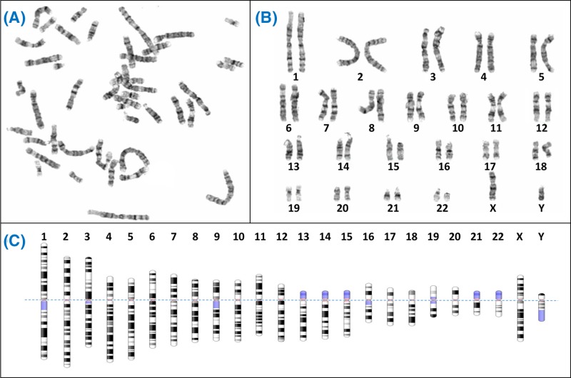
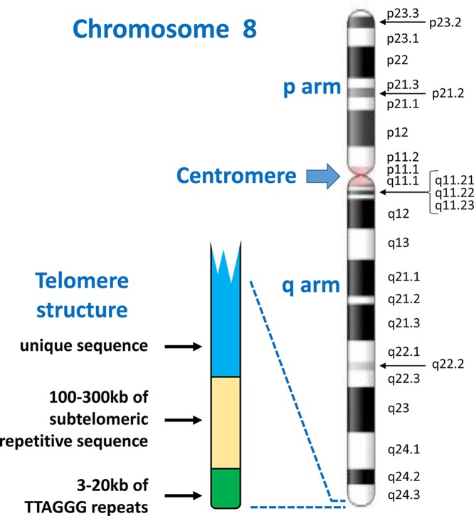
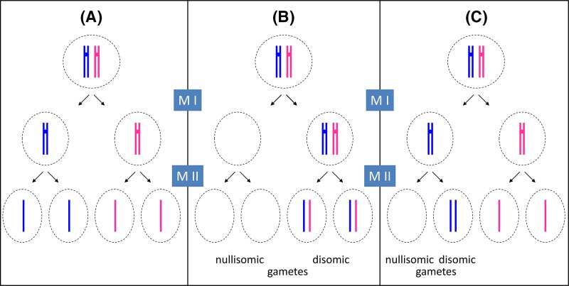
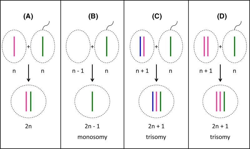
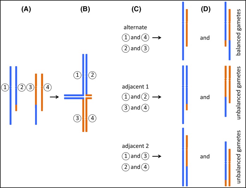
Chromosome structure and chromosomal disorders

    1. To learn more about general genetics, consult one of many available text books. The following is freely available online.
    1. Griffiths A.J.F, Miller J.H., Suzuki D.T., Lewontin R.C. and Gelbart W.M. (2000) An Introduction to Genetic Analysis, 7th edn, W.H. Freeman, New York, https://www.ncbi.nlm.nih.gov/books/NBK21766/

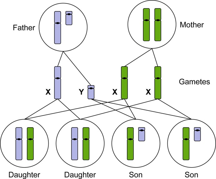
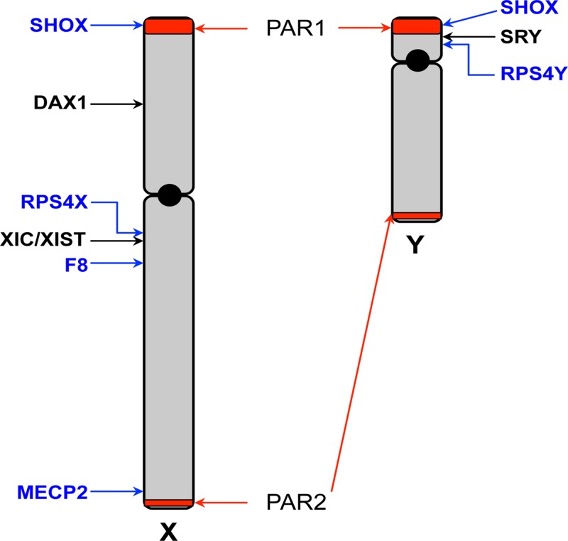
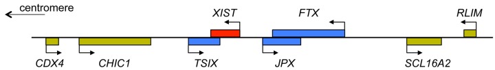
The sex chromosomes, X and Y

    1. Bonora G. and Disteche C.M. (2017) Structural aspects of the inactive X chromosome. Phil. Trans. R. Soc. B Biol. Sci. 372, 20160357, (and others in this volume of 12 contributions to a discussion meeting issue ‘X-chromsome inactivation: a tribute to Mary Lyon’) 10.1098/rstb.2016.0357 - DOI - PMC - PubMed
    1. Fiot E., Zenaty D., Boizeau P., Haignere J., Dos Santos S. and Leger J (2016) X-chromosome gene dosage as a determinant of impaired pre and postnatal growth and adult height in Turner syndrome. Eur. J. Endocrinol. 174, 281–288 10.1530/EJE-15-1000 - DOI - PubMed
    1. Gamble T. and Zarkower D. (2012) Sex determination. Current Biol. 22:, 257–262 10.1016/j.cub.2012.02.054 - DOI - PMC - PubMed
    1. Gilbert S.F. (2000) Developmental Biology, 6th edn, Chromosomal Sex Determination in Mammals Sinauer Associates
    1. Lombardi L.M., Baker S.A. and Zoghbi H.Y. (2015) MECP2 disorders: from the clinic to mice and back. J. Clin. Invest. 125, 2914–2923 10.1172/JCI78167 - DOI - PMC - PubMed

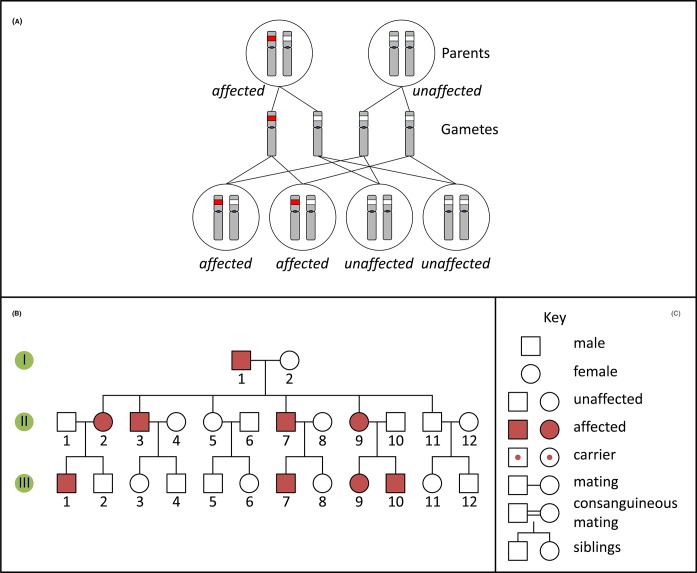
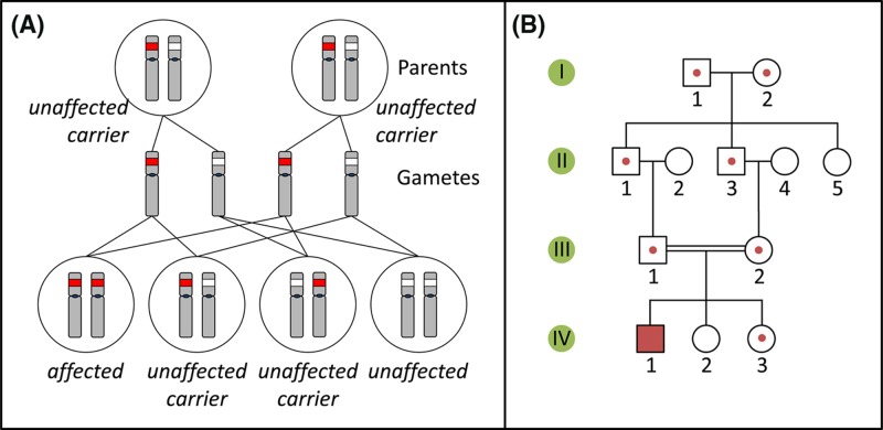
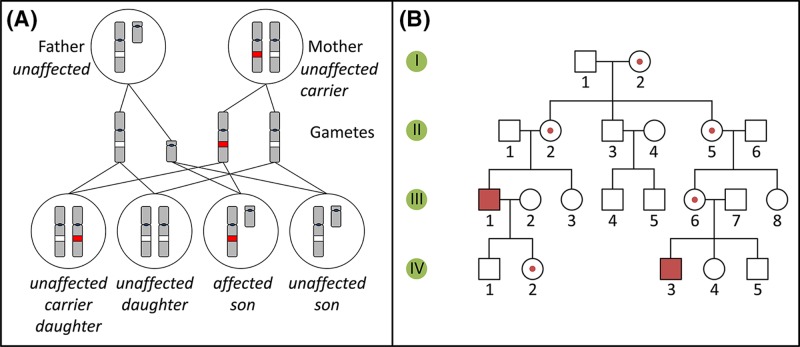
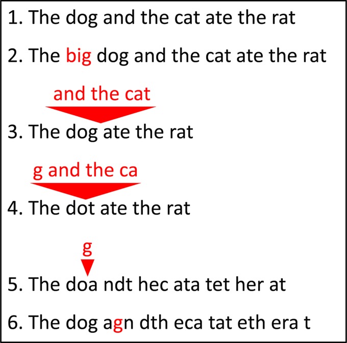
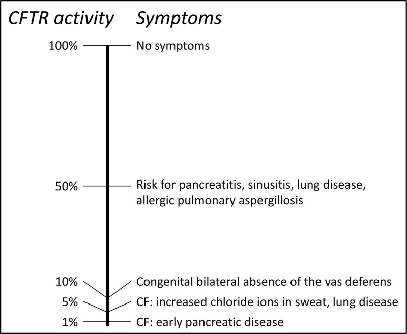
Single-gene disorders

    1. Chial H. (2008) Mendelian genetics: patterns of inheritance and single-gene disorders. Nat. Education 1, 63
    1. Davis P.B. (2001) Cystic fibrosis. Pediatr. Rev. 22, 257–264 10.1542/pir.22-8-257 - DOI - PubMed
    1. Martiniano S.L., Sagel S.D. and Zemanick E.T. (2016) Cystic fibrosis: a model system for precision medicine. Curr. Opin. Pediatr. 28:, 312–317 10.1097/MOP.0000000000000351 - DOI - PMC - PubMed
    1. Nopoulos P.C. (2016) Huntington disease: a single-gene degenerative disorder of the striatum. Dialogues Clin. Neurosci. 18, 91–98 - PMC - PubMed
    1. Ornitz D.M. and Legeai-Mallet L. (2017) Achondroplasia: development, pathogenesis, and therapy. Dev. Dyn. 246, 291–309 10.1002/dvdy.24479 - DOI - PMC - PubMed

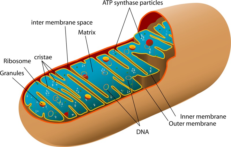
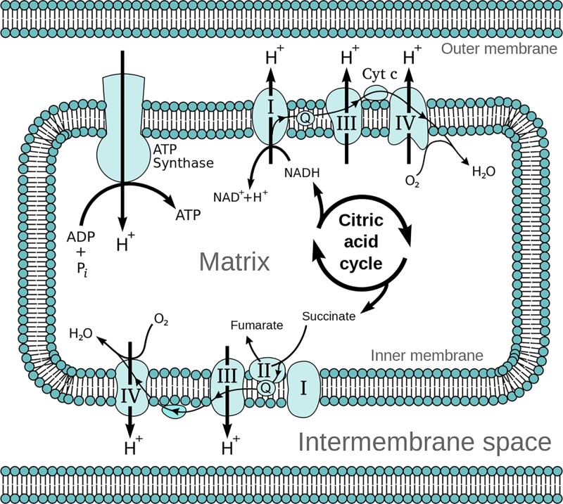
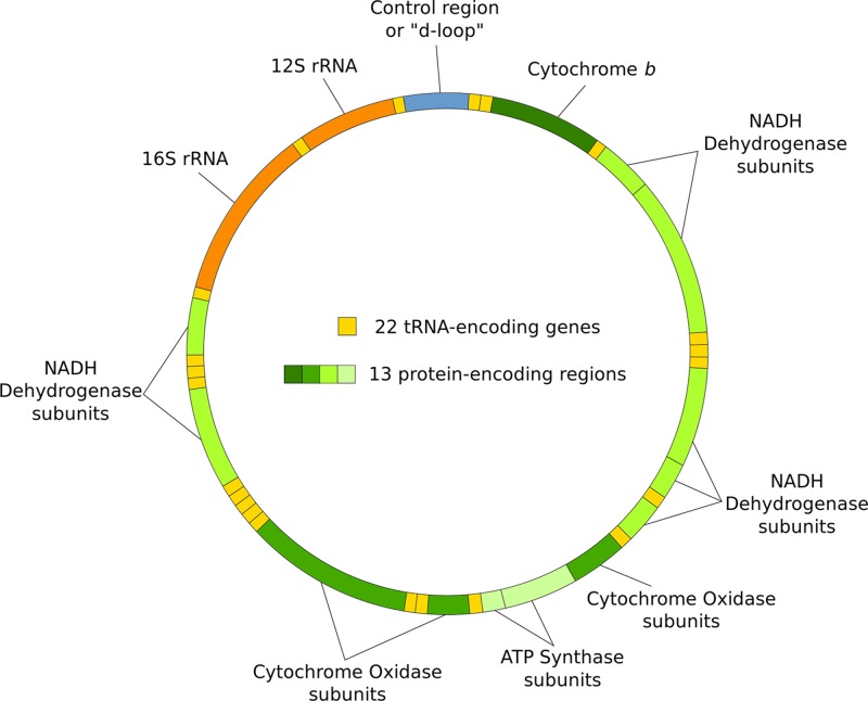
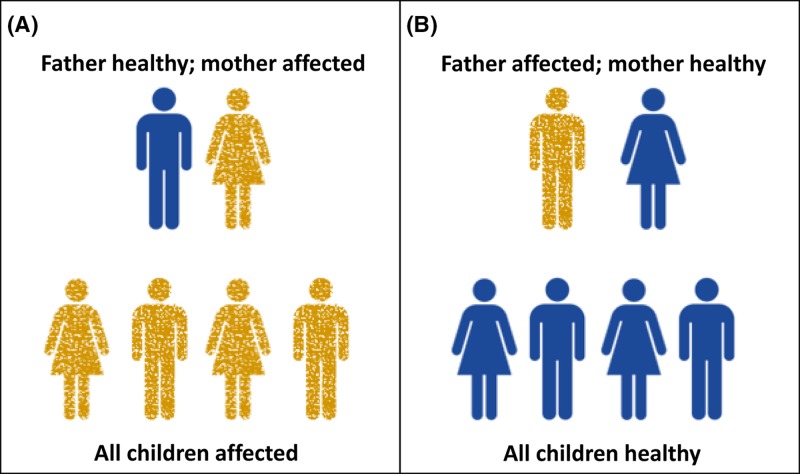
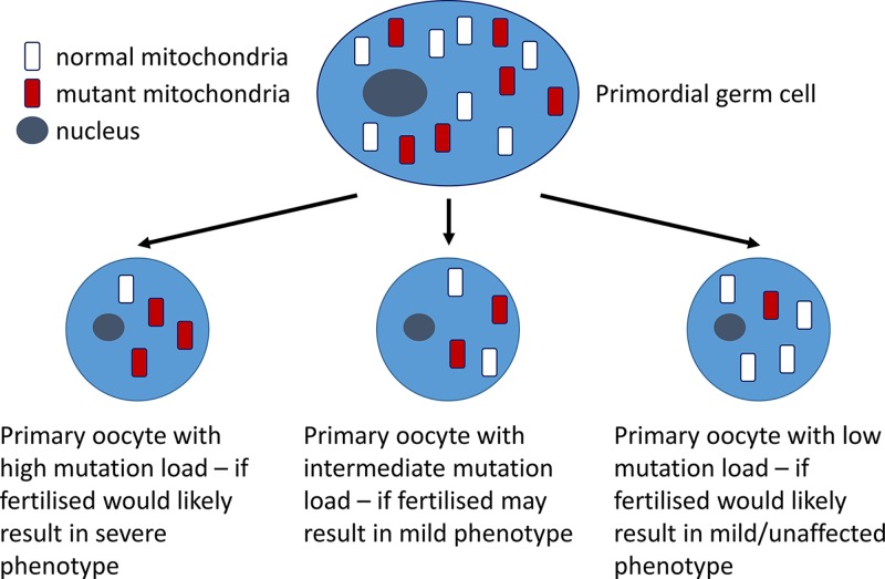
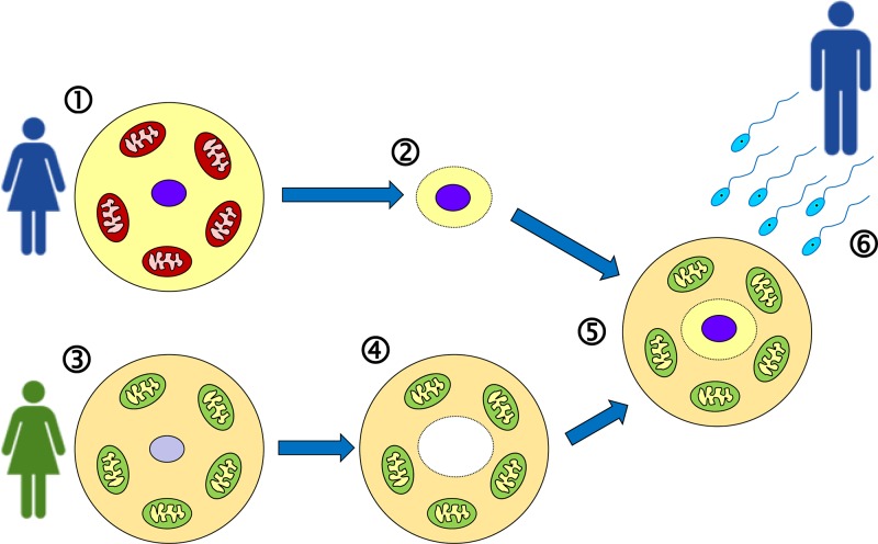
Mitochondrial disorders

    1. Chinnery P. (2000) Mitochondrial Disorders Overview. SourceGeneReviews® (Adam M.P., Ardinger H.H., Pagon R.A., Wallace S.E., Bean L.J.H., Stephens K. and Amemiya A., eds), pp. 1993–2018, University of Washington, Seattle, Seattle (WA)
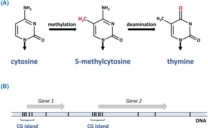
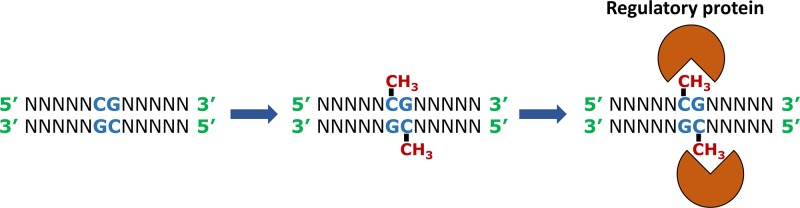
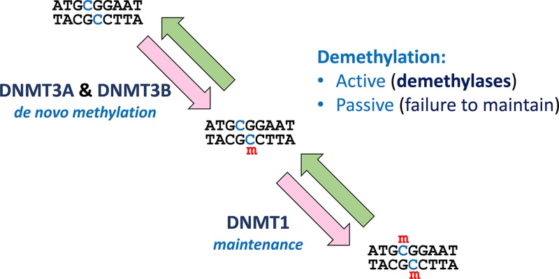
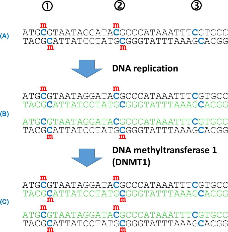
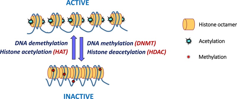
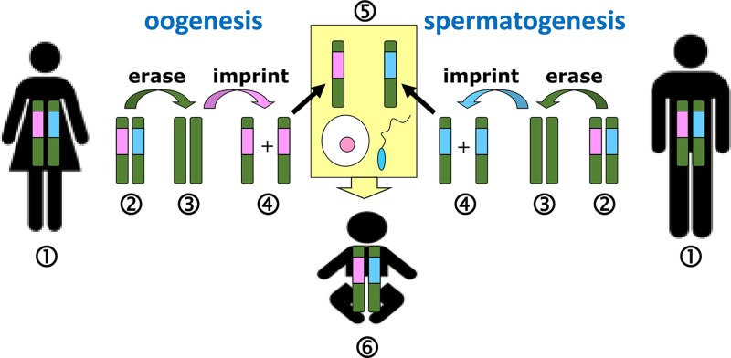
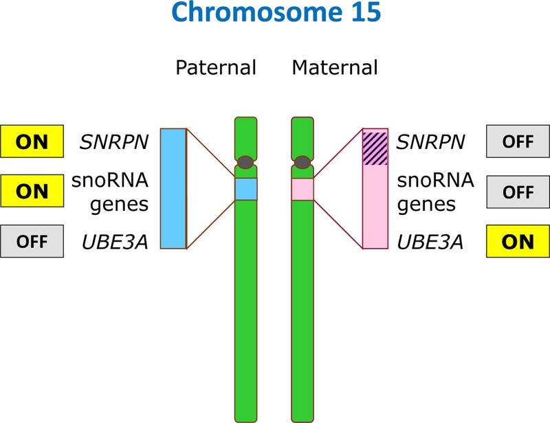
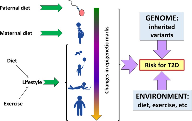
    1. Chong J.X., Buckingham K.J., Jhangiani S.N., Boehm C., Sobreira N., Smith J.D.. et al. (2015) The genetic basis of mendelian phenotypes: discoveries, challenges, and opportunities. Am. J. Hum. Genet. 97, 199–215 10.1016/j.ajhg.2015.06.009 - DOI - PMC - PubMed
    1. Nightingale H., Pfeffer G., Bargiela D., Horvath R. and Chinnery P. F. (2016) Emerging therapies for mitochondrial disorders. Brain 139, 1633–1648 10.1093/brain/aww081 - DOI - PMC - PubMed
    1. Reznichenko A., Huyser C. and Pepper M. (2016) Mitochondrial transfer: implications for assisted reproductive technologies. Appl. Transl. Genom. 11, 40–47 10.1016/j.atg.2016.10.001 - DOI - PMC - PubMed

Epigenetics

    1. Barlow D.P. and Bartolomei M.S. (2014) Genomic imprinting in mammals. Cold Spring Harb. Perspect. Biol. 6, a018382 10.1101/cshperspect.a018382 - DOI - PMC - PubMed
    1. Lobo I. (2008) Genomic imprinting and patterns of disease inheritance. Nat. Education 1, 66
    1. Schuebel K., Gitil M., Domschke K. and Goldman D. (2016) Making sense of epigenetics. Int. J. Neuropsychopharmacol. 19, 1–10 10.1093/ijnp/pyw058 - DOI - PMC - PubMed
    1. Soshnev A.A., Josefowicz S.Z. and Allis C.D. (2016) Greater than the sum of parts: complexity of the dynamic epigenome. Mol. Cell 62, 681–694 10.1016/j.molcel.2016.05.004 - DOI - PMC - PubMed
    1. Venturá-Junca P., Irarrázaval I., Rolle A.J., Gutiérrez J.I., Moreno R.D. and Santos M.J. (2015) In vitro fertilization (IVF) in mammals: epigenetic and developmental alterations. Scientific and bioethical implications for IVF in humans. Biol. Res. 48:, 68 10.1186/s40659-015-0059-y - DOI - PMC - PubMed
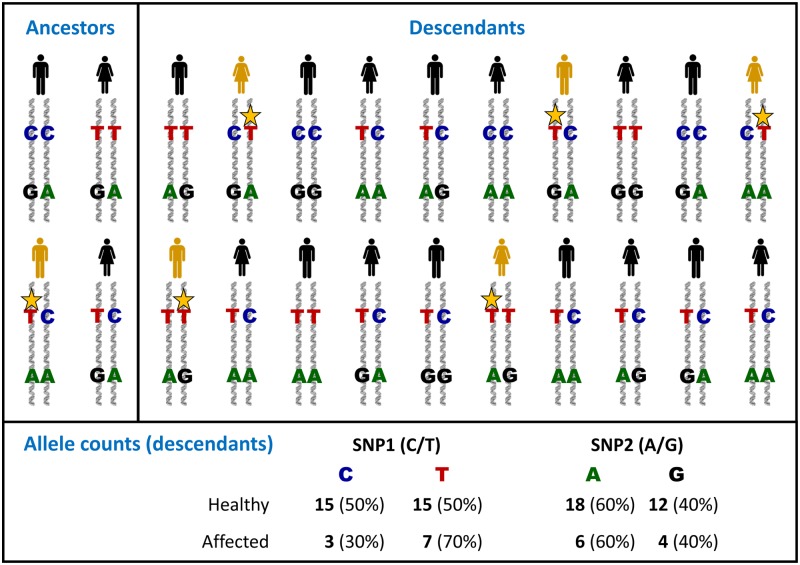
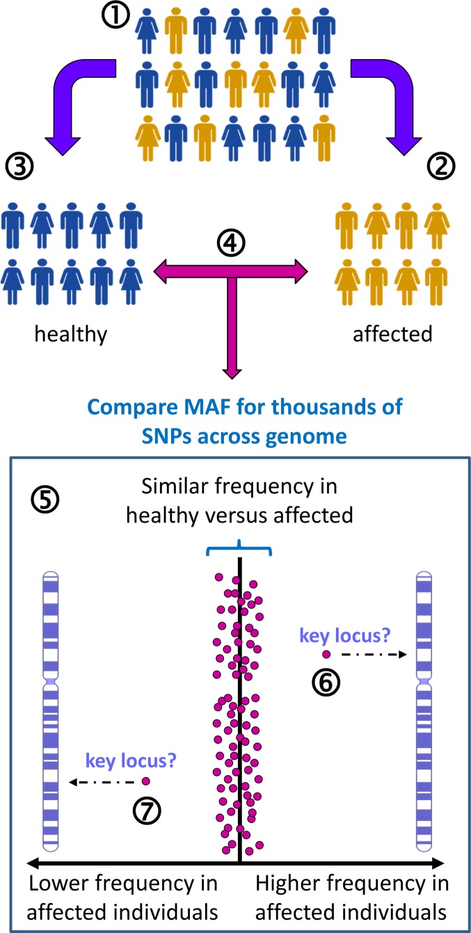
Complex disorders

    1. Chial H. and Craig J. (2008) Genome-wide association studies (GWAS) and obesity. Nat. Education 1, 80
    1. Prasad R.B. and Groop L. (2015) Genetics of type 2 diabetes–pitfalls and possibilities. Genes 6, 87–123 10.3390/genes6010087 - DOI - PMC - PubMed
    1. Schulz L.C. (2010) The Dutch Hunger Winter and the developmental origins of health and disease. Proc. Natl. Acad. Sci. U.S.A. 107, 16757–16758 10.1073/pnas.1012911107 - DOI - PMC - PubMed

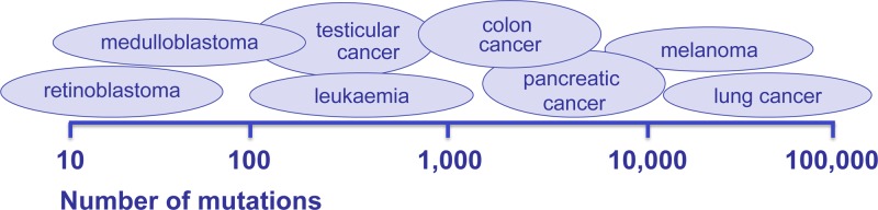
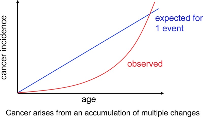
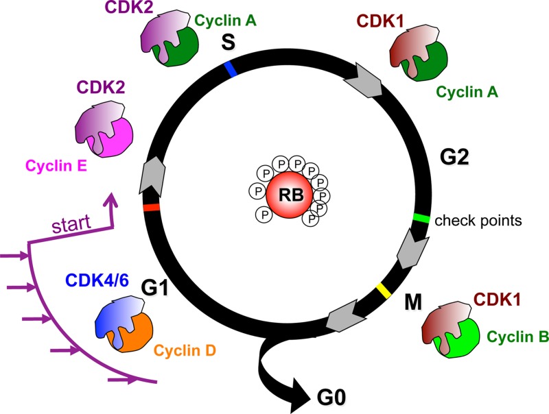
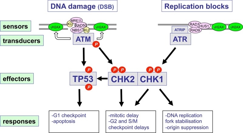
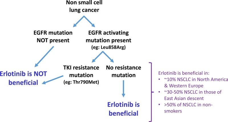
Cancer: mutation and epigenetics
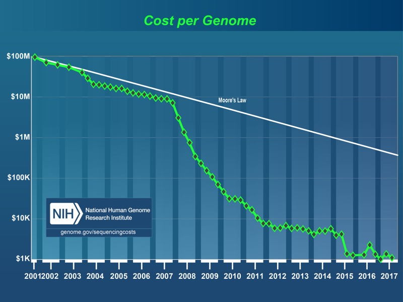
    1. Aunan J.R., Cho W.C. and Søreide K. (2017) The biology of aging and cancer: a brief overview of shared and divergent molecular hallmarks. Aging Dis. 8, 628–642 10.14336/AD.2017.0103 - DOI - PMC - PubMed
    1. Burotto M., Chiou V.L., Lee J-M. and Kohn E.C. (2014) The MAPK pathway across different malignancies: A new perspective. Cancer 120, 3446–3456 10.1002/cncr.28864 - DOI - PMC - PubMed
    1. Delbridge A.R., Valente L.J. and Strasser A. (2012) The role of the apoptotic machinery in tumor suppression. Cold Spring Harb. Perspect. Biol. 4, a008789. - PMC - PubMed
    1. Feinberg A.P., Koldobskiy M.A. and Gondor A. (2016) Epigenetic modulators, modifiers and mediators in cancer aetiology and progression. Nat. Rev. Genet. 17, 284–299 10.1038/nrg.2016.13 - DOI - PMC - PubMed
    1. Fischer M. and Müller G.A. (2017) Cell cycle transcription control: DREAM/MuvB and RB-E2F complexes. Crit. Rev. Biochem. Mol. Biol. 52, 638–662 10.1080/10409238.2017.1360836 - DOI - PubMed

Genomics

    1. Feero W.G. and Gutmacher A.E. (2014) Genomics, personalized medicine, and paediatrics. Acad. Pediatr. 14, 14–22 10.1016/j.acap.2013.06.008 - DOI - PMC - PubMed
    1. Genomics England, 100,000 genomes project, 2018. https://www.genomicsengland.co.uk/
    1. Naidoo N., Pawitan Y., Soong R., Cooper D.N. and Ku C.-S. (2011) Human genetics and genomics a decade after the release of the draft sequence of the human genome. Hum. Genomics 5, 577–622 10.1186/1479-7364-5-6-577 - DOI - PMC - PubMed
    1. Rehm H.L. (2017) Evolving healthcare through personal genomics. Nat. Rev. Genet. 18, 259–267 10.1038/nrg.2016.162 - DOI - PMC - PubMed
    1. Scottish Genomes Partnership (2018), https://www.scottishgenomespartnership.org/

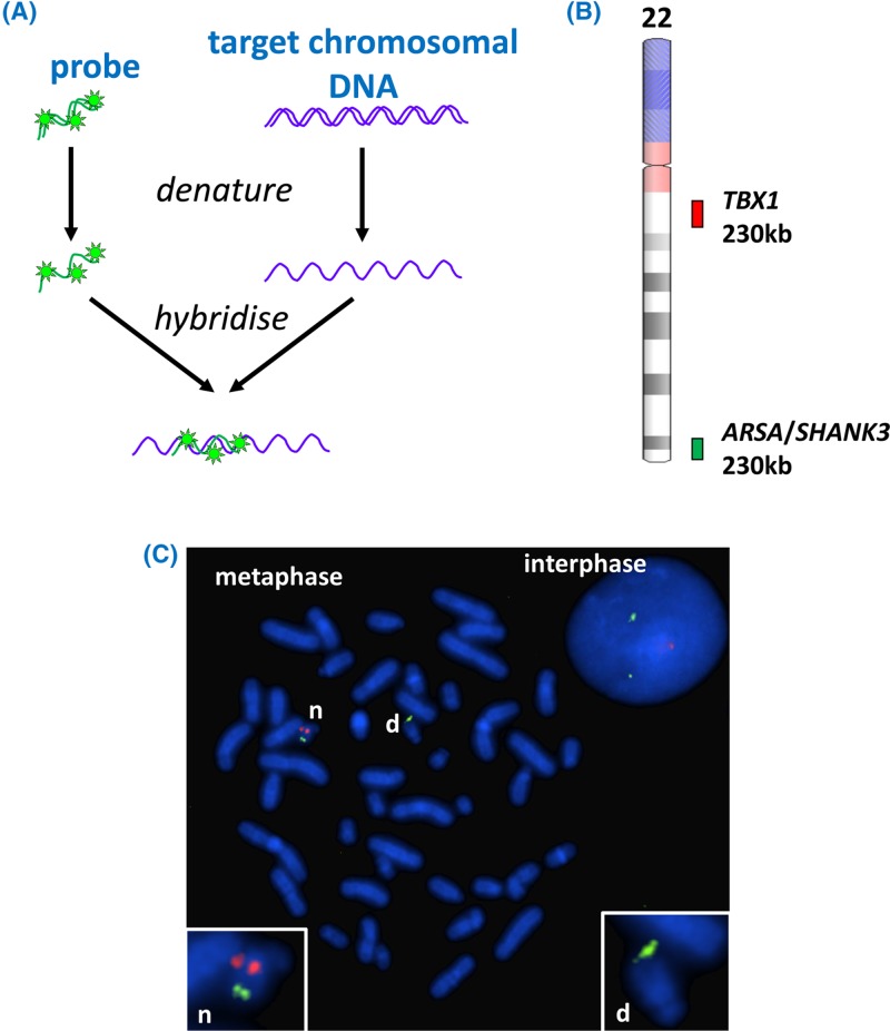
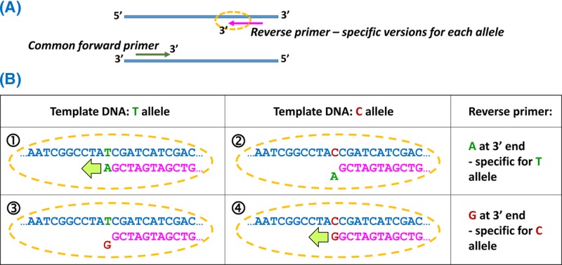
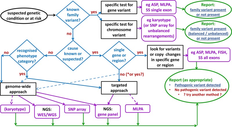
Genetic testing in the diagnostic laboratory

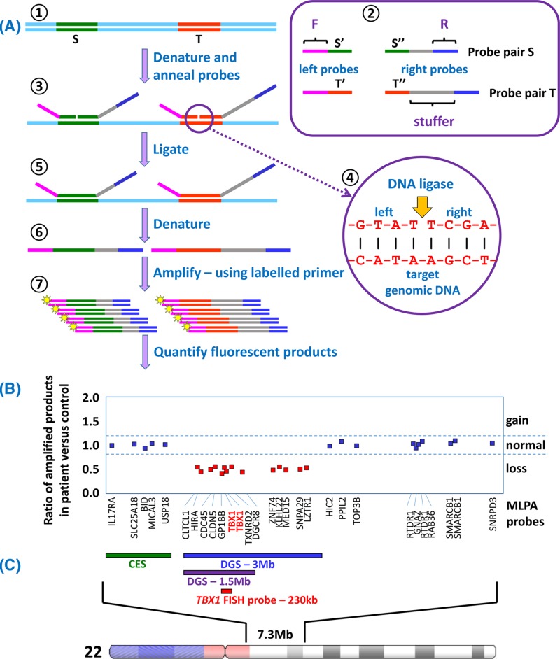
    1. Bishop R. (2010) Applications of fluorescence in situ hybridization (FISH) in detecting genetic aberrations of medical significance. Biosci. Horiz. 3, 85–95, 10.1093/biohorizons/hzq009 - DOI
    1. Ferrie R.M., Schwarz M.J., Robertson N.H., Vaudin S., Super M., Malone G.. et al. (1992) Development, multiplexing, and applications of ARMS tests for common mutations in the CFTR gene. Am. J. Hum. Genet. 51, 251–262 - PMC - PubMed
    1. Frese K.S., Katus H.A. and Meder B. (2013) Next-generation sequencing: from understanding biology to personalized medicine. Biology (Basel) 2, 378–398 - PMC - PubMed
    1. Katsanis S.H. and Katsanis N. (2013) Molecular genetic testing and the future of clinical genomics. Nat. Rev. Genet. 14, 415–426 10.1038/nrg3493 - DOI - PMC - PubMed
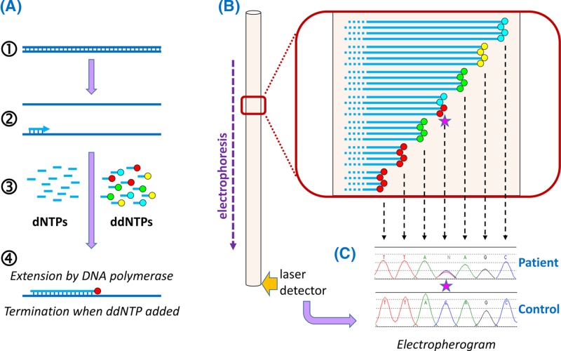
    1. Kchouk M., Gibrat J.-F. and Elloumi M. (2017) Generations of sequencing technologies: from first to next generation. Biol. Med. (Aligarh) 9, 395 10.4172/0974-8369.1000395 - DOI

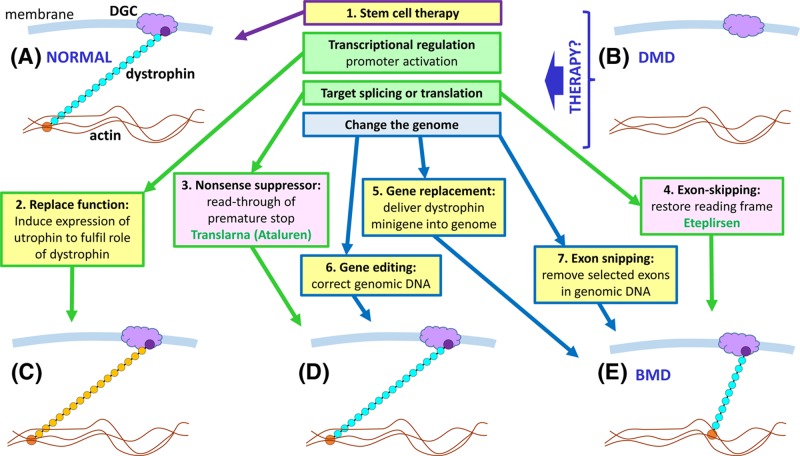
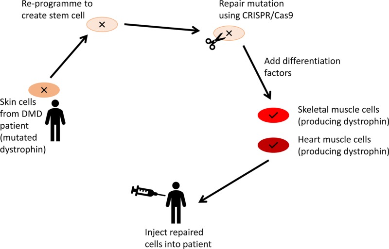
Diagnosis, management and therapy of genetic disease

    1. Aronson S.J. and Rehm H.L. (2015) Building the foundation for genomics in precision medicine. Nature 526, 336–342 10.1038/nature15816 - DOI - PMC - PubMed
    1. Chaterji S., Ahn E.H. and Kim D.-H. (2017) CRISPR genome engineering for human pluripotent stem cell research. Theranostics 7, 4445–4469 10.7150/thno.18456 - DOI - PMC - PubMed
    1. Eid A. and Mahfouz M.M. (2016) Genome editing: the road of CRISPR/Cas9 from bench to clinic. Exp. Mol. Med. 48, e265 10.1038/emm.2016.111 - DOI - PMC - PubMed
    1. Lockyer E. (2016) The potential of CRISPR-Cas9 for treating genetic disorders. Biosci. Horiz. 9, 10.1093/biohorizons/hzw012 - DOI
    1. Martiniano S.L., Sagel S.D. and Zemanick E.T. (2016) Cystic fibrosis: a model system for precision medicine. Curr. Opin. Pediatr. 28, 312–317 10.1097/MOP.0000000000000351 - DOI - PMC - PubMed

Challenges in delivering a genetics service

    1. Blashki G., Metcalfe S. and Emery J. (2014) Genetics in general practice. Aust. Fam. Phys. 43, 428–431 - PubMed
    1. Harris A., Kelly S. E. and Wyatt S. (2013) Counseling customers: emerging roles for genetic counselors in the direct-to-consumer genetic testing market. J. Genet. Couns. 22, 277–288 10.1007/s10897-012-9548-0 - DOI - PMC - PubMed
    1. Roberts J.S., Dolinoy D. and Tarini B. (2014) Emerging issues in public health genomics. Annu. Rev. Genomics Hum. Genet. 15, 461–480 10.1146/annurev-genom-090413-025514 - DOI - PMC - PubMed
    1. Su P. (2013) Direct-to-consumer genetic testing: a comprehensive view. Yale J. Biol. Med. 86, 359–365 - PMC - PubMed