Three-dimensional texture analysis of optical coherence tomography images of ovarian tissue

Abstract

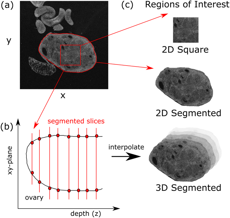
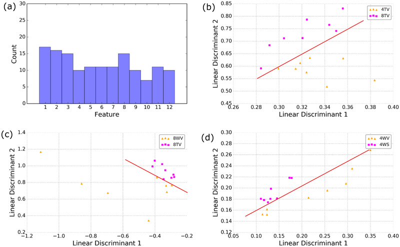
Ovarian cancer has the lowest survival rate among all gynecologic cancers due to predominantly late diagnosis. Optical coherence tomography (OCT) has been applied successfully to experimentally image the ovaries in vivo; however, a robust method for analysis is still required to provide quantitative diagnostic information. Recently, texture analysis has proved to be a useful tool for tissue characterization; unfortunately, existing work in the scope of OCT ovarian imaging is limited to only analyzing 2D sub-regions of the image data, discarding information encoded in the full image area, as well as in the depth dimension. Here we address these challenges by testing three implementations of texture analysis for the ability to classify tissue type. First, we test the traditional case of extracted 2D regions of interest; then we extend this to include the entire image area by segmenting the organ from the background. Finally, we conduct a full volumetric analysis of the image volume using 3D segmented data. For each case, we compute features based on the Grey-Level Co-occurence Matrix and also by introducing a new approach that evaluates the frequency distribution in the image by computing the energy density. We test these methods on a mouse model of ovarian cancer to differentiate between age, genotype, and treatment. The results show that the 3D application of texture analysis is most effective for differentiating tissue types, yielding an average classification accuracy of 78.6%. This is followed by the analysis in 2D with the segmented image volume, yielding an average accuracy of 71.5%. Both of these improve on the traditional approach of extracting square regions of interest, which yield an average classification accuracy of 67.7%. Thus, applying texture analysis in 3D with a fully segmented image volume is the most robust approach to quantitatively characterizing ovarian tissue.

Figure 1.

The ovaries are manually segmented from the image background, selecting regions of interest (ROIs) both as square areas and as the entire ovary (a). The segmentation is done throughout the tissue depth (b), which is then interpolated to yield the 3D segmentation. This gives rise to three types of ROIs: 2D square, 2D segmented and 3D segmented (c).

Figure 2.

The GLCM is constructed by measuring the probability of two pixel values i and j occurring a distance d from one another (a). This can be done for four different directions in 2D (b), and thirteen directions total for 3D (c).

Figure 3.

The frequency analysis is done by integrating the fractional energy in a disk centered at the origin of coordinates for the FFT (a). The radius of the disk is increased until reaching 80% of the maximum value. For the 3D case, the disk becomes an ellipse, scaled by the axis lengths in x, y and z (b).

Figure 4.

Representative features from the 2d application of the GLCM. The parameters of angular second moment (a), correlation (b), variance (c) and inverse difference moment (d) proved to be the most statistically significant for differentiating the mouse groups. Error bars are given by the standard deviation of the result evaluated over the population of mice. Significance levels are represented by a triangles for age groups, + for genotypes and * for treatments, with one and two symbols for p <0.05 and p < 0.01, respectively.

Figure 5.

Representative features from the 3D application of the GLCM. Entropy is a powerful feature for differentiating all groups (a). Individually, difference variance (b) is useful for age, while difference entropy is powerful for treatment (c) and sum average provides statistical significance for genotype (d). Error bars are given by the standard deviation of the result evaluated over the population of mice. Significance levels are represented by a triangles for age groups, + for genotypes and * for treatments, with one and two symbols for p <0.05 and p < 0.01, respectively.

Figure 6.

Representative images of the ovaries for mice at 4 weeks treated with sesame oil for wild type (a) and TAg (b) genotypes. There is very little observable differences between the two, leading to very similar texture features. In contrast, wild type (c) and TAg (d) mice at 8 weeks while treated with VCD show clear differences, reflected in the variation among texture features.

Figure 7.

The energy density is distributed differently as a function of frequency for different mouse groups, for example 4 week (magenta + symbols) and 8 week (orange dots) wild type mice treated with VCD. Fitting these curves to a two-parameter model yields an additional two features for analysis. The curves shown here are for the 3D analysis

Figure 8.

Frequency analysis results for 2D (a,b) and 3D (c,d). In both cases, the distribution is described using two parameters: α (a,c) and β (b,d). Error bars are given by the standard deviation of the result evaluated over the population of mice. Significance levels are represented by a triangles for age groups, + for genotypes and * for treatments, with one, two, and three symbols for p <0.05, p < 0.01, and p <0.0001, respectively.

Figure 9.

Histogram of the frequency with which features were selected (a). From the best features, the linear discriminants were computed and the data were projected onto these axes. Examples for which the data can be separated with high accuracy with only 2 linear discriminants for age (b), genotype (c) and treatment (d). Red lines are a visual aid to illustrate the axis of discrimination.

References

1. Abdolmanafi A, Duong L, Dahdah N, Cheriet F, 2017. Deep feature learning for automatic tissue classification of coronary artery using optical coherence tomography. Biomed. Opt. Express 8, 1203 URL: https://www.osapublishing.org/DirectPDFAccess/F77DD5AD-0BC7-36D6-5C4AA46..., doi:10.1364d/BOE.8.001203. - DOI - PMC - PubMed
1. Abràmoff M, Garvin MK, Sonka M, 2010. Retinal imaging and image analysis. IEEE Rev. Biomed. Eng 1, 169–208. URL: http://ieeexplore.ieee.org/xpls/abs_all.jsp?arnumber=5660089, doi:10.1109/RBME.2010.2084567.Retinal. - DOI - PMC - PubMed
1. Barnholtz-Sloan JS, Schwartz AG, Qureshi F, Jacques S, Malone J, Munkarah AR, 2003. Ovarian cancer: Changes in patterns at diagnosis and relative survival over the last three decades. Am. J. Obstet. Gynecol 189, 1120–1127. doi:10.1067/S0002-9378(03)00579-9. - DOI - PubMed
1. Bast RC, 2003. Status of tumor markers in ovarian cancer screening. doi:10.1200/JCO.2003.01.068. - DOI - PubMed
1. Beauvoit B, Evans SM, Jenkins TW, Miller EE, Chance B, 1995. Correlation between the light scattering and the mitochondrial content of normal tissues and transplantable rodent tumors. Anal. Biochem 226, 167–174. doi:10.1006/abio.1995.1205. - DOI - PubMed