Community dynamics and sensitivity to model structure: towards a probabilistic view of process-based model predictions

Abstract

Statistical inference and mechanistic, process-based modelling represent two philosophically different streams of research whose primary goal is to make predictions. Here, we merge elements from both approaches to keep the theoretical power of process-based models while also considering their predictive uncertainty using Bayesian statistics. In environmental and biological sciences, the predictive uncertainty of process-based models is usually reduced to parametric uncertainty. Here, we propose a practical approach to tackle the added issue of structural sensitivity, the sensitivity of predictions to the choice between quantitatively close and biologically plausible models. In contrast to earlier studies that presented alternative predictions based on alternative models, we propose a probabilistic view of these predictions that include the uncertainty in model construction and the parametric uncertainty of each model. As a proof of concept, we apply this approach to a predator-prey system described by the classical Rosenzweig-MacArthur model, and we observe that parametric sensitivity is regularly overcome by structural sensitivity. In addition to tackling theoretical questions about model sensitivity, the proposed approach can also be extended to make probabilistic predictions based on more complex models in an operational context. Both perspectives represent important steps towards providing better model predictions in biology, and beyond.

Keywords: Bayesian statistics; community dynamics; model predictions; predation; structural sensitivity.

Figure 1.

Results of the Markov chain Monte Carlo estimate of parameters probability densities (posterior distributions) for each function. (a–c) Bivariate posterior probability distributions (grey levels) for each functional response parameter, i.e. the likelihood of these parameter values based on available data. Points ‘+’ correspond to parameter values sampled to perform the probabilistic model analysis. Black bullets (one per panel) indicate the parameter values with the maximum likelihood, i.e. parameter values giving the best fit to data. (d–f) Functional responses fit to experimental data (points ‘+’). The parametric uncertainty from the HMCMC estimation gives a confidence interval (95%, shaded area) around the best-fitted functions (curves). Model uncertainty is derived through the relative likelihood that one function fits new data better than the others, knowing their respective parametric uncertainty. (Online version in colour.)

Figure 2.

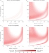
Probabilistic predictions of Rosenzweig–MacArthur model, made with each alternative functional response (a–c) and averaged (d). Probabilistic predictions include both parametric uncertainty for each function (a–c), and model uncertainty for the average prediction (d). Each panel presents a probabilistic bifurcation diagram, where the colours indicate the qualitative system dynamics depending on the predator mortality rate and the prey carrying capacity: predator extinction (white), prey–predator coexistence at equilibrium (blue), prey–predator oscillations (green) and bistability with equilibrium coexistence or oscillations depending on initial population sizes (red). Colour gradients indicate the probability (red-green-blue levels) of each model predictions. Thus, blurred areas (e.g. top left of panel (d)) indicate uncertain predictions. Calculations at point ‘+’ are detailed in table 2. (Online version in colour.)

Figure 3.

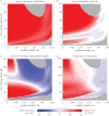
Uncertainty in predictions made with the Rosenzweig–MacArthur model. Details of the calculations if one chooses to use Holling functional response: uncertainty due to functional response’s parameter values (a), to the choice of the functional response (b), and their sum (c). (d) Total uncertainty (like in (c)) averaged over the three alternative functional responses, weighted by their respective likelihood. Calculations at point ‘+’ are detailed in table 2. (Online version in colour.)

Figure 4.

Source of uncertainty in predictions made with the Rosenzweig–MacArthur model. Relative importance of parametric (negative value, blue) and model (positive value, red) uncertainty in the resulting total predictive uncertainty (grey area: total prediction uncertainty lower than 0.01). (a–c) Source of uncertainty if one of the alternative functional responses is chosen. (d) Average over the three alternative functions, weighted by their respective likelihood. Calculations at point ‘+’ are detailed in table 2. (Online version in colour.)

Figure 5.

Example where one equation is almost certainly the best one among candidates. Overview of the analysis with data on copepods (Calanus pacificus) feeding on diatoms (centric sp.). All panels are drawn similarly as in earlier figures: (a) functional responses are fitted to data by a HMCMC algorithm; (b) average qualitative predictions (probabilistic bifurcation diagram); (c) average total uncertainty in predictions; (d) source of uncertainty in predictions.

Figure 6.

Example where all alternative equations are equally likely. Overview of the analysis with data on starved copepods (Calanus pacificus) feeding on diatoms (Thalassiosira fluviatilis). All panels are drawn similarly as in earlier figures: (a) functional responses are fitted to data by a HMCMC algorithm; (b) average qualitative predictions (probabilistic bifurcation diagram); (c) average total uncertainty in predictions; (d) source of uncertainty in predictions. Note that here we took K_max as five times the maximum prey density in data, in order to show all the possible qualitative dynamics predicted by the model, without altering our conclusions. (Online version in colour.)

References

1. Anderson TR. 2010. Progress in marine ecosystem modelling and the ‘unreasonable effectiveness of mathematics’. J. Mar. Sys. 81, 4–11. (10.1016/j.jmarsys.2009.12.015) - DOI
1. Petchey OL. et al. 2015. The ecological forecast horizon, and examples of its uses and determinants. Ecol. Lett. 18, 597–611. (10.1111/ele.12443) - DOI - PMC - PubMed
1. Pennekamp F, Adamson MW, Petchey OL, Poggiale JC, Aguiar M, Kooi BW, Botkin DB, DeAngelis DL. 2017. The practice of prediction: what can ecologists learn from applied, ecology-related fields? Ecol. Complexity 32, 156–167. (10.1016/j.ecocom.2016.12.005) - DOI
1. Baker RE, Peña JM, Jayamohan J, Jérusalem A. 2018. Mechanistic models versus machine learning, a fight worth fighting for the biological community? Biol. Lett. 14, 20170660 (10.1098/rsbl.2017.0660) - DOI - PMC - PubMed
1. Rosenzweig ML, MacArthur RH. 1963. Graphical representation and stability conditions of predator–prey interaction. Am. Nat. 97, 209–223. (10.1086/282272) - DOI
Publication types