Population coding of valence in the basolateral amygdala

Abstract

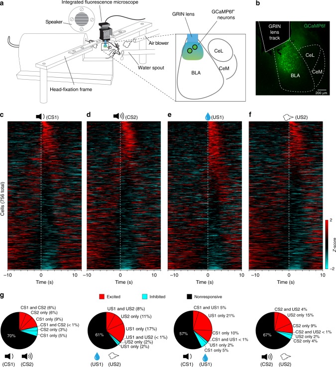
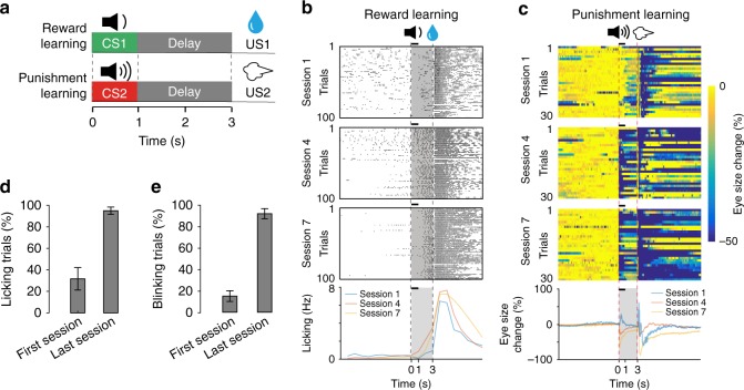
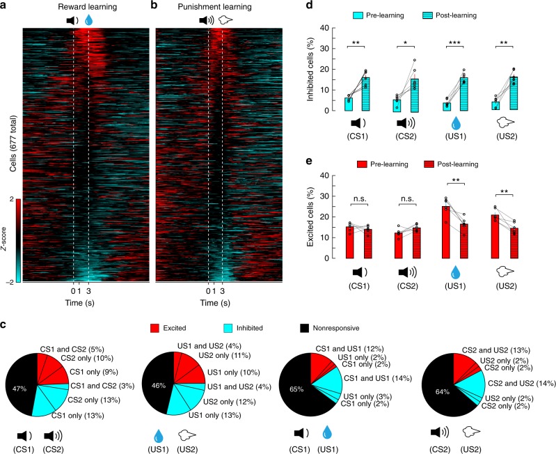
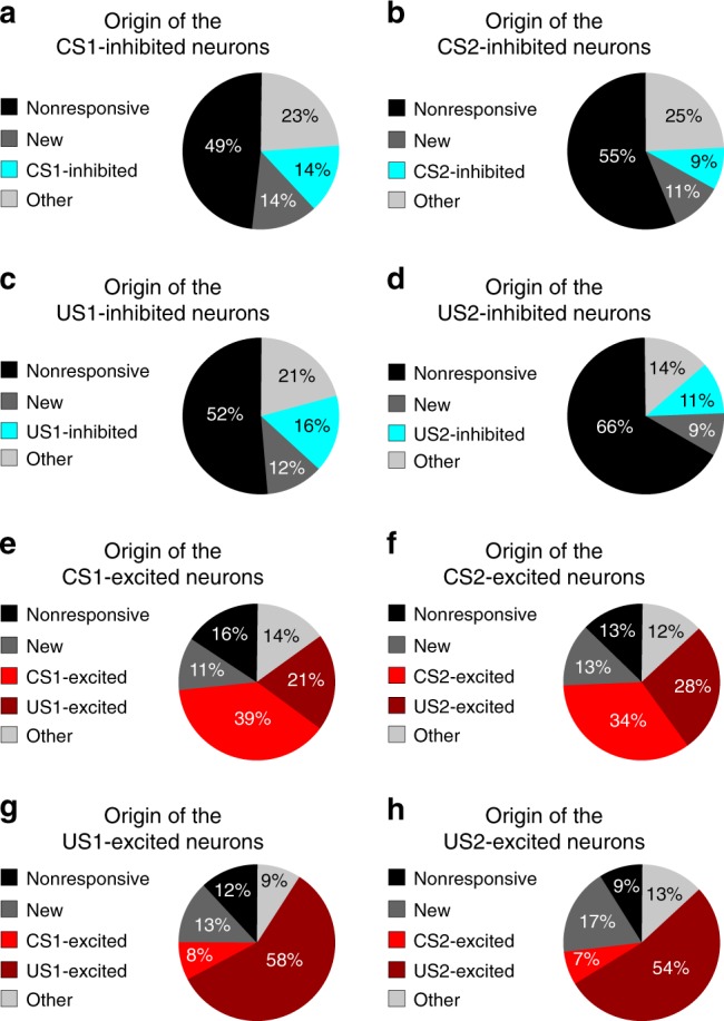
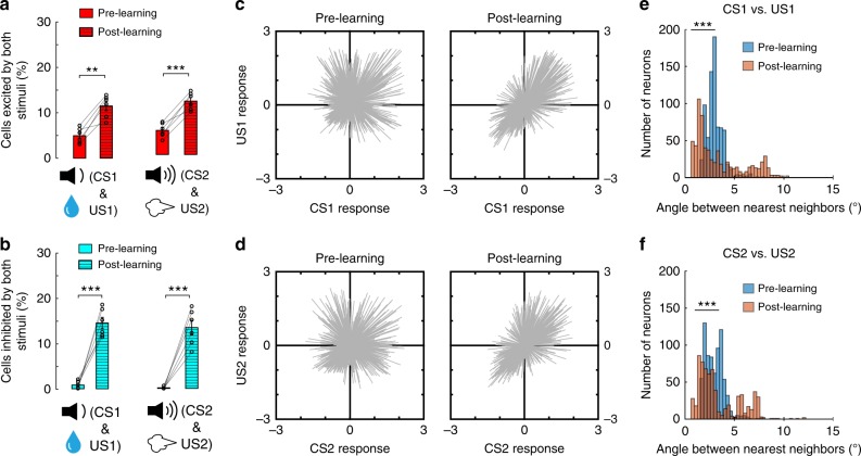
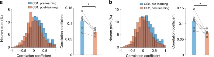
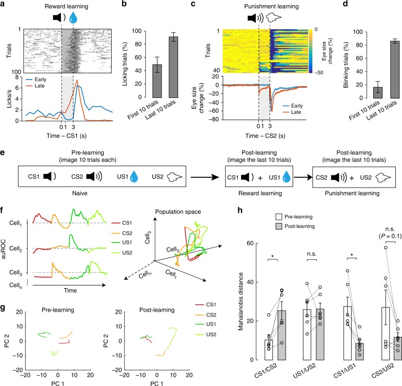
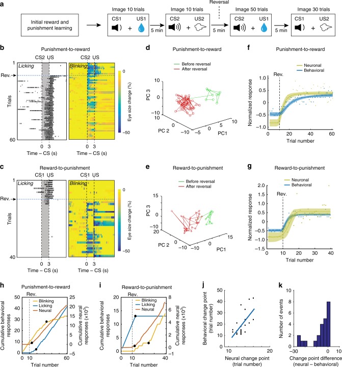
The basolateral amygdala (BLA) plays important roles in associative learning, by representing conditioned stimuli (CSs) and unconditioned stimuli (USs), and by forming associations between CSs and USs. However, how such associations are formed and updated remains unclear. Here we show that associative learning driven by reward and punishment profoundly alters BLA population responses, reducing noise correlations and transforming the representations of CSs to resemble the valence-specific representations of USs. This transformation is accompanied by the emergence of prevalent inhibitory CS and US responses, and by the plasticity of CS responses in individual BLA neurons. During reversal learning wherein the expected valences are reversed, BLA population CS representations are remapped onto ensembles representing the opposite valences and predict the switching in valence-specific behaviors. Our results reveal how signals predictive of opposing valences in the BLA evolve during learning, and how these signals are updated during reversal learning thereby guiding flexible behaviors.

Fig. 1

The innate responses of BLA neurons to CSs and USs. a A schematic of the setup for simultaneously monitoring behavioral and neuronal responses in head-restrained mice. We imaged GCaMP6 signals in BLA neurons through GRIN lenses in behaving mice using a miniature integrated fluorescence microscope mounted on the head. b A representative confocal image of a coronal brain section containing the BLA, in which the track of an implanted GRIN lens was on top of the BLA neurons expressing GCaMP6f. c Heatmaps of the activities (z-scores) for all neurons (n = 756 neurons, six mice) in trials in which CS1 was presented (indicated by the dashed line). Each row represents the temporal activities of one neuron. Neurons are sorted according to their average z-scores during the 1-s time window immediately after CS1 onset. d–f Same as (c), except that CS2 (d), US1 (water reward) (e), or US2 (air-puff) (f) was presented as the stimulus. g Pie charts showing the percent distributions of neurons responsive to different stimuli before learning. Note that at this stage, inhibitory responses were rare; and only a small percentage of neurons responded to both CS1 and US1, or to both CS2 and US2

Fig. 2

The behavioral task. a A schematic of the behavioral procedure, in which mice were trained to associate CS1 (a 2 kHz tone) with US1 (water reward), and CS2 (a 10 kHz tone) with US2 (air-puff blowing to the face). b Changes in licking behavior during the reward learning for a representative mouse. The upper three panels are raster plots of licking events during early (session 1), mid (session 4), and late (session 7) training stages. The bottom panel shows average licking rate over time (1-s bin) for each of the three sessions in the upper panels. Licks are aligned to the onset of CS1 (t = 0; the duration of CS1 (1 s) is indicated by a black bar above each panel). The delivery of US1 (water) was at 3 s after CS1 onset. Licks in the shaded area represent predictive licking events. c Eye blinking, measured as eye size change over time (see Methods), during the punishment learning for the same mouse as that in (b). The upper three panels are heat-maps of eye blinking during early (session 1), mid (session 4), and late (session 7) training stages. The bottom panel shows average blinking over time for each of the three sessions in the upper panels. Eye blinks are aligned to CS2 onset (t = 0; the duration of CS2 (1 s) is indicated by a black bar above each panel). The delivery of US2 (air-puffs) was at 3 s after CS2 onset. Eye blinks in the shaded area represent predictive blinking events. d and e The percentage of trials in which mice showed predictive licking (d) or blinking (e) (i.e., trials with at least one lick (d) or blink (e) event in the shaded area) in the first and last training sessions (the first 10 trials of each session were used for analysis) (n = 6 mice)

Fig. 3

The CS and US responses in BLA neurons after learning. BLA neuronal activities were imaged in mice (n = 6) well trained with both the reward and the punishment conditioning. a Left: heatmaps of activities (z-scores) for all neurons (n = 677) in the reward block, in which CS1 was paired with US1 (indicated by the dashed lines). Each row represents the temporal activities of one neuron. Neurons are sorted according to their average z-scores during the 0–1 s time window. b Same as (a), except that imaging was performed in the punishment block, in which CS2 was paired with US2. c Pie charts showing the percent distributions of neurons responsive to different stimuli after learning. Note that at this stage, inhibitory responses became prominent; and the percentage of neurons responsive to both CS1 and US1, or to both CS2 and US2 increased. d Proportions of BLA neurons showing inhibitory responses to the CSs and USs before and after learning (N = 6 mice; CS1, t₍₅₎ = −5.075, **P = 0.0039; CS2, t₍₅₎ = −3.393, *P = 0.0194; US1, t₍₅₎ = −9.413, ***P = 2.28e−4; US2, t₍₅₎ = −5.886, **P = 0.002; paired t-test). e Proportions of BLA neurons showing excitatory responses to the CSs and USs before and after learning (CS1, t₍₅₎ = 0.83, P = 0.44; CS2, t₍₅₎ = −1.18, P = 0.29; US1, t₍₅₎ = 5.24, **P = 0.003; US2, t₍₅₎ = 4.194, **P = 0.008; paired t-test)

Fig. 4

The origin of post-learning CS-responsive and US-responsive neurons. a–d For the BLA neurons showing inhibitory responses to CS1 (a), CS2 (b), US1 (c), or US2 (d) at the post-learning stage, the majority of them did not respond at the pre-learning stage to any of these stimuli (“nonresponsive”); some of them were not identified (“new”), were originally inhibited by CS1 (a), CS2 (b), US1 (c), or US2 (d) or were responsive to other stimuli (“other”) at the pre-learning stage. e, f For the BLA neurons showing excitatory responses to CS1 (e) or CS2 (f) at the post-learning stage, some of them did not respond at the pre-learning stage to any stimuli (“nonresponsive”); some of them were not identified (“new”), were originally excited by CS1 (“CS1-excited”) or US1 (“US1-excited”) (e) or by CS2 (“CS2-excited”) or US2 (“US2-excited”) (f), or were responsive to other stimuli (“other”) at the pre-learning stage. (g, h) For the BLA neurons showing excitatory responses to US1 (g) or US2 (h) at the post-learning stage, the majority of them were originally excited by US1 (“US1-excited”) (g) or US2 (“US2-excited”) (h) at the pre-learning stage; some of them did not respond to any stimuli (“nonresponsive”), were not identified (“new”), were originally excited by CS1 (“CS1-excited”) (g) or CS2 (“CS2-excited”) (h), or were responsive to other stimuli (“other”) at the pre-learning stage

Fig. 5

Learning links CS and US representations in the BLA. a The percentage of BLA neurons showing excitatory responses to both CS and US (n = 6 mice; CS1 & US1, t₍₅₎ = −6.116, **P = 0.0017; CS2 and US2, t₍₅₎ = −9.2, ***P = 2.5e−4; paired t-test). b The percentage of BLA neurons showing inhibitory responses to both CS and US (n = 6 mice; CS1 and US1, t₍₅₎ = −8.8, ***P = 3.12e−4; CS2 and US2, t₍₅₎ = −8.3, ***P = 4.11e−4; paired t-test). c, d The responses to CS1 and US1 (c), or to CS2 and US2 (d), for each neuron. Each line is a vector representing the responses of a particular neuron to both the CS and the US (values represent z-scores). Note that before learning, the vectors are distributed uniformly in the four quadrants, whereas after learning, the vectors are more concentrated in quadrants I and III. e The distribution of angles between the nearest neighbors among vectors in (c) (pre-learning median, 3.89, n = 756 neurons, post-learning median, 2.36, n = 677 neurons, z = 4.73, ***P = 2.26e−6, rank sum test). f The distribution of angles between the nearest neighbors among vectors in (d) (pre-learning median, 3.93, n = 756 neurons, post-learning median, 2.60, n = 677 neurons, z = 5.3, ***P = 1.42e−7, rank sum test)

Fig. 6

Learning reduces noise correlations in the BLA. a Left, histograms of noise correlations in the responses to CS1 in BLA neurons in a representative mouse. Right, comparison of noise correlations between pre-learning and post-learning conditions (n = 6 mice, t₍₅₎ = 3.2, *P = 0.0241, paired t-test). b Left, histograms of noise correlations in the responses to CS2 in BLA neurons in a representative mouse. Right, comparison of noise correlations between pre-learning and post-learning conditions (n = 6 mice, t₍₅₎ = 3.04, *P = 0.0288, paired t- test). The bar graphs on the right in a and b represent mean ± s.e.m

Fig. 7

Learning transforms CS representations in the BLA. a Changes in licking during the reward learning for a representative mouse. Upper panel: raster plot of licking events across trials. Bottom panel: average licking rate over time (1-s bin), plotted separately for early and late trials. Dashed lines indicate the onsets of CS1 (1 s duration) and US1 (water). Licks in the shaded area represent predictive licking events. b The percentage of trials in which mice showed predictive licking in the first and last 10 trials (n = 3 mice). c Changes in eye blinking during the punishment learning for the same mouse as that in (a). Upper panel: heat-maps of eye size changes across trials. Bottom panel: average eye size changes over time, plotted separately for early and late trials. Dashed lines indicate the onsets of CS2 (1 s duration) and US2 (air-puff). Eye blinks in the shaded area represent predictive blinking events. d The percentage of trials in which mice showed predictive blinking in the first and last 10 trials (n = 3 mice). e The timing of the imaging experiments relative to behavioral training. f Left: a schematic of the population vector analysis. The dynamic activities of a neuron (cell₁–cell_n for each mouse) during the 1 s time window immediately after the onset of each stimulus (CS1, CS2, US1, or US2) are represented by a vector, which is composed of sequential frame-by-frame z-scores computed for that neuron. Right: the trajectory of a population vector for three example neurons in a 3D space. g The BLA population activity from one representative mouse. The first two principal components before (left) and after (right) learning are projected onto a 2D space. h Quantification of the Mahalanobis distances between vectors representing neuronal responses to different stimuli (n = 6 mice; CS1/CS2, t₍₅₎ = −3.25, *P = 0.022; US1/US2, t₍₅₎ = −0.07, P = 0.94 (n.s., nonsignificant); CS1/US1, t₍₅₎ = 3.29, *P = 0.021; CS2/US2, t₍₅₎ = 2.01; P = 0.1; paired t-test). Data are presented as mean ± s.e.m

Fig. 8

Population BLA activities correlate and predict behavioral responses during reversal learning. a A schematic showing the experimental procedure. The imaging procedure was designed such that no detachment/reattachment of the camera was needed, allowing ambiguous tracking of the same neurons throughout the reversal learning. b Punishment-to-reward reversal learning. Simultaneous measuring of licking (left) and blinking (right) behavior in the 10 trials before and 50 trials after the valence associated with CS2 changed from negative to positive. The horizontal dashed line denotes the first trial (11th trial) at which the valence was reversed. c Reward-to-punishment reversal learning. Simultaneous measuring of licking (left) and blinking (right) behavior in the 10 trials before and 30 trials after the valence associated with CS1 changed from positive to negative. The horizontal dashed line denotes the first trial (11th trial) at which the valence was reversed. d, e Projection of the trial-by-trial CS population responses (from 677 neurons) onto a 3D PCA space, in the punishment-to-reward (d) and the reward-to-punishment (e) reversal learning. f, g Average normalized neuronal and behavioral responses plotted as a function of trial number, for punishment-to-reward (f) and reward-to-punishment (g) reversal learning. f Fitting for behavioral responses, r² = 0.86, fitting for neuronal responses, r² = 0.83, Pearson correlation coefficient between behavioral and neuronal responses, r = 0.96, P < 0.001. g Fitting for behavioral responses, r² = 0.91, fitting for neuronal responses, r² = 0.74, Pearson correlation coefficient between behavioral and neuronal responses, r = 0.98, P < 0.001. Each of the dashed lines indicates the first trial (11th) at which the reversal of a CS valence has occurred. Shaded areas indicate 95% prediction intervals for Weibull fitting (n = 6 mice). h, i Cumulative plot of trial-by-trial measures of behavioral (licking and blinking) and neural responses of one representative animal in punishment-to-reward (h) and reward-to-punishment (i) reversal learning. Neural responses are represented as Mahalanobis distances between vectors representing the population CS response in a trial and a vector distribution that represents the population CS responses in all the 10 trials before the reversals (see text; also see f, g). Black dots represent the change points. j Correlation between behavioral change points and neural change points (r² = 0.42, P = 6.3e−4, Pearson correlation). The blue line is the regression line. k Histogram showing the difference between neural and behavioral change points

References

1. Cardinal RN, Parkinson JA, Hall J, Everitt BJ. Emotion and motivation: the role of the amygdala, ventral striatum, and prefrontal cortex. Neurosci. Biobehav. Rev. 2002;26:321–352. doi: 10.1016/S0149-7634(02)00007-6. - DOI - PubMed
1. Davis M. Anatomic and physiologic substrates of emotion in an animal model. J. Clin. Neurophysiol. 1998;15:378–387. doi: 10.1097/00004691-199809000-00002. - DOI - PubMed
1. LeDoux JE. Emotion circuits in the brain. Annu. Rev. Neurosci. 2000;23:155–184. doi: 10.1146/annurev.neuro.23.1.155. - DOI - PubMed
1. Rosen JB. The neurobiology of conditioned and unconditioned fear: a neurobehavioral system analysis of the amygdala. Behav. Cogn. Neurosci. Rev. 2004;3:23–41. doi: 10.1177/1534582304265945. - DOI - PubMed
1. Schultz W. Behavioral theories and the neurophysiology of reward. Annu. Rev. Psychol. 2006;57:87–115. doi: 10.1146/annurev.psych.56.091103.070229. - DOI - PubMed
Publication types