Visual stimulus-driven functional organization of macaque prefrontal cortex

Abstract

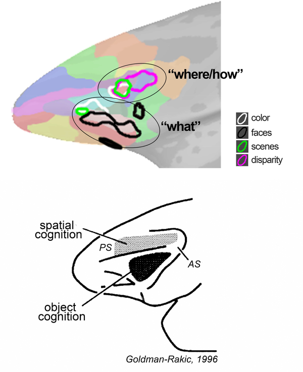
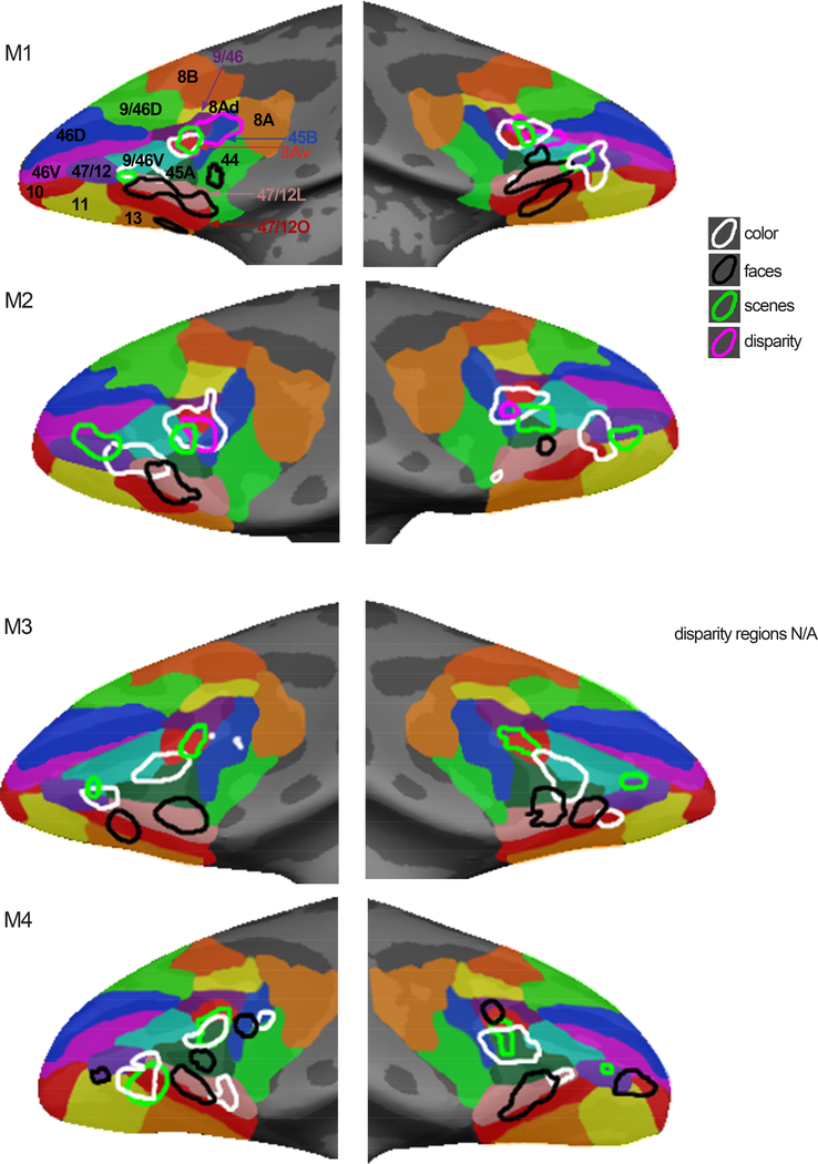
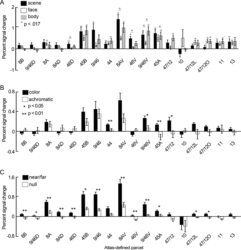
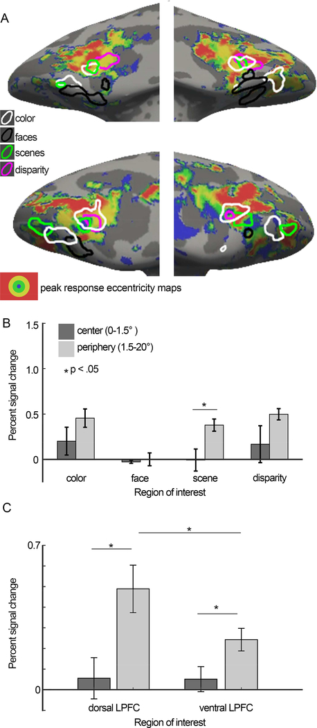
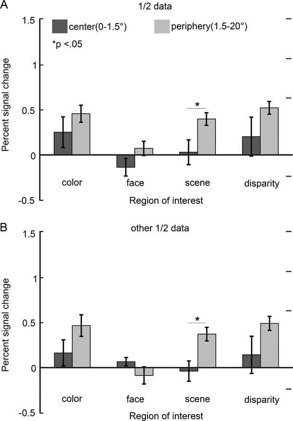
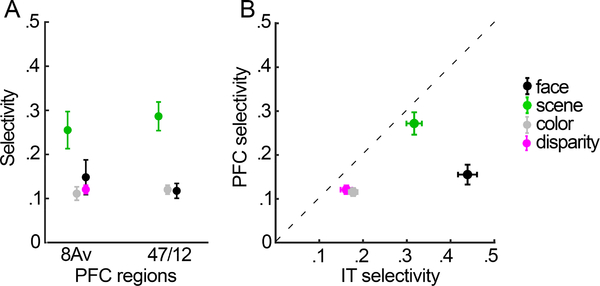
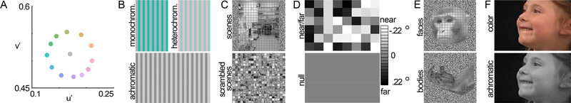
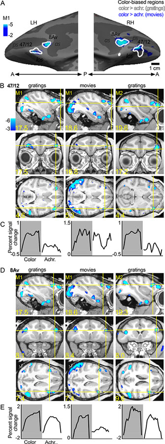
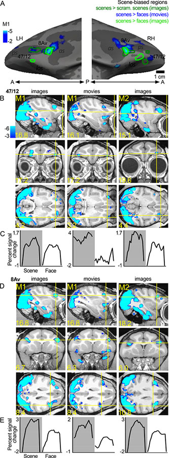
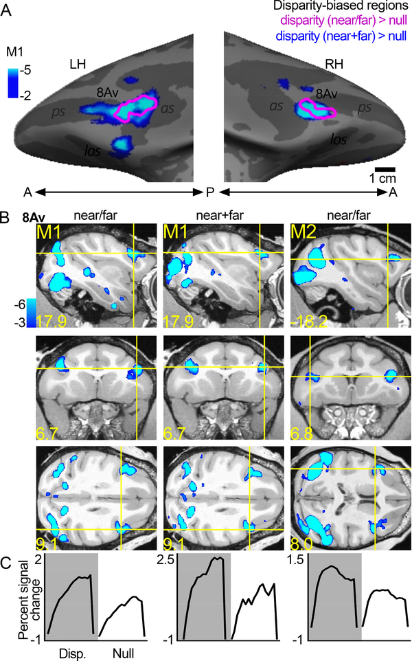
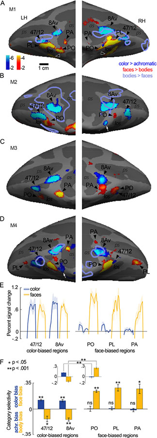
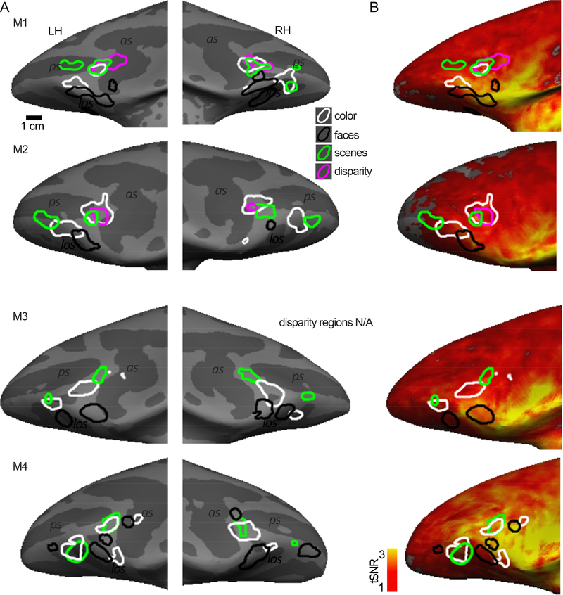
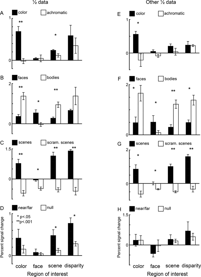
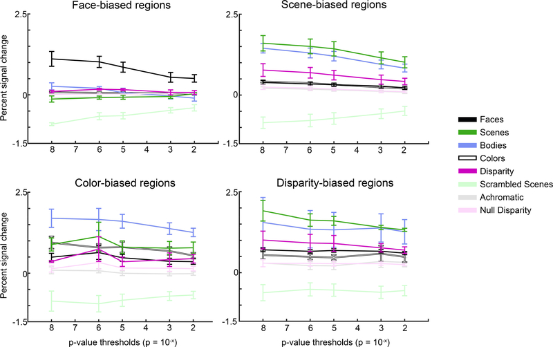
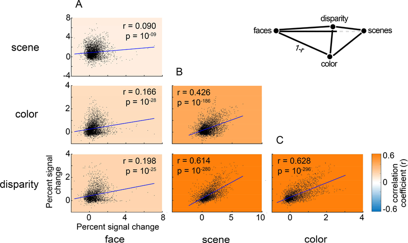
The extent to which the major subdivisions of prefrontal cortex (PFC) can be functionally partitioned is unclear. In approaching the question, it is often assumed that the organization is task dependent. Here we use fMRI to show that PFC can respond in a task-independent way, and we leverage these responses to uncover a stimulus-driven functional organization. The results were generated by mapping the relative location of responses to faces, bodies, scenes, disparity, color, and eccentricity in four passively fixating macaques. The results control for individual differences in functional architecture and provide the first account of a systematic visual stimulus-driven functional organization across PFC. Responses were focused in dorsolateral PFC (DLPFC), in the ventral prearcuate region; and in ventrolateral PFC (VLPFC), extending into orbital PFC. Face patches were in the VLPFC focus and were characterized by a striking lack of response to non-face stimuli rather than an especially strong response to faces. Color-biased regions were near but distinct from face patches. One scene-biased region was consistently localized with different contrasts and overlapped the disparity-biased region to define the DLPFC focus. All visually responsive regions showed a peripheral visual-field bias. These results uncover an organizational scheme that presumably constrains the flow of information about different visual modalities into PFC.

Figure 1.. Stimuli used to assess the visual stimulus-driven functional organization of prefrontal cortex in macaque monkeys.

A. Chromaticities of the 12 colors used in the monochromatic gratings. B. Color stimuli were configured as low spatial frequency gratings, either monochromatic (color-gray) or heterochromatic (defined by the cardinal and intermediate directions of color space). Voxels were defined as color biased if they showed stronger responses to colored gratings than to achromatic luminance-contrast gratings. Note that the “gray” phase of the color-gray gratings appears reddish in the figure because of color induction; the gray itself was defined as the neutral adapting state of the null conditions. C. Scene stimuli consisted of photographs of the lab environment. Responses to scene stimuli were contrasted with responses to scrambled versions of the scene images, or with responses to faces. D. Schematic of the disparity stimulus, which consisted of random-dot anaglyph stereogram checkerboards (see scale bar). Responses were contrasted against null-disparity random-dot patterns. E. Face stimuli consisted of photographs of monkey faces. Responses were contrasted with responses to bodies. F. Dynamic stimuli consisted of short video clips showing faces, scenes, objects and bodies, presented either in color or grayscale.

Figure 2.. Color-biased regions in prefrontal cortex of macaque monkey.

A. Color-biased activity in animal M1 shown on the computationally inflated cortical surface, lateral views (LH, left hemisphere; RH, right hemisphere; P, posterior; A, anterior). The blue-cyan significance map shows the color > luminance activity for the dynamic movie stimuli (color movies > achromatic movies). The white contours show color > luminance responses measured with colored gratings. Color-biased activations were only found in lateral PFC extending into orbital PFC, in or near anatomically defined parcels 8Av and 47/12. B. Sagittal (top), coronal (middle), and horizontal (bottom) slices showing the responses to color, using gratings and movie clips; slices centered on 47/12, in two monkeys (M1 and M2; surface maps for M1 shown in panel A). Blue-cyan significance maps for each condition are superimposed on high-resolution anatomical scans of each animal’s own anatomy. Slices are labeled in Talairach coordinates (mm). C. Time course of the average percent signal change in the color-biased region of interest shown in panel B (time course and ROI defined using in independent datasets). Stimulus blocks were 16 TRs (2sec/TR; 32sec/block) for gratings stimuli and 15 TRs (2sec/TR; 30sec/block) for movie stimuli. As in B, the left column shows the time course for M1 as measured with gratings stimuli, the middle column shows responses to movies stimuli in M1, and the right column shows activations to gratings stimuli in M2. D, E. Same conventions as in B and C, for the more posterior color-biased region, in or near area 8Av. as, arcuate sulcus; ps, principal sulcus; los, lateral orbital sulcus.

Figure 3.. Scene-biased regions in prefrontal cortex of macaque monkey.

A. Scene-biased activity in animal M1 shown on the computationally inflated cortical surface. The blue-cyan significance map shows the scene > face activity using responses to movie clips. The dark green contours show scene > scrambled scene activity measured with responses to static images. The light green contour shows scene > faces measured with static images. Scene-biased activity was consistently found across contrasts in or near 8Av. B. Slices showing the scene-biased activation in two images and movies, in M1 and M2. C. Time course of the average percent signal change in the 47/12 scene-biased region, as measured in independent datasets. D, E. Same conventions as in B and C, for the posterior scene-biased region, in or near area 8Av. Other conventions as for Figure 2.

Figure 4.. Disparity-biased region in prefrontal cortex of macaque monkey.

A. Disparity-biased activity in monkey M1 shown on the computationally inflated cortical surface. The blue-cyan significance map shows disparity > null disparity responses measured with disparity stimuli that in any given block contained only near or far disparity checks. The magenta contours show regions of disparity > null activity measured in other experiments, using disparity checkerboards containing both near and far depths (near+far) presented simultaneously. With both stimulus sets, a disparity-biased region was identified in both hemispheres, in or near anatomical parcel 8Av. B. Slices showing disparity activity in the two conditions and two animals (M1 and M2). C. Time course of the average percent signal change observed in the disparity-biased region of interest; ROI was defined with data independent of the data used to quantify the time course. Other conventions as for Figure 2.

Figure 5.. Relationship between color-biased and face-biased regions of frontal cortex of macaque monkey.

A-D Inflated prefrontal cortex surfaces of four animals (M1-M4). Significance maps showing color > luminance (gratings) in blue-cyan and faces > bodies (images) in yellow-red are displayed. E. Time courses of the average percent signal change observed for color and face stimuli in the color-biased regions (left plot, in or near anatomical parcels 47/12 and 8Av), and the prefrontal face-biased regions (right panel); the face-biased regions are labeled following published conventions (PO, PL, PA). Time courses were generated using data that were independent of the data used to define the regions of interest. Shading shows SEM. F. Quantification of color and face selectivity, using data that was independent of the data used to define the regions of interest. Color regions show a bias for color and bodies, while face regions show a bias for faces and no color bias. Each bar represents the mean activity as calculated across all hemispheres for which a region was present: 47/12r, 8 hemispheres; 8Av, 8 hemispheres; PA, 6 hemispheres; PL, 6 hemispheres; PO, 7 hemispheres. Error bars show the SEM. Inset shows results averaged across color ROIs (left panel) and face ROIs (right panel). Color responses were greater in color ROIs than in face ROIs (p=10⁻⁴); face biased response were greater in face ROI.

Figure 6.. Spatial relationship between regions of interest, and tSNR maps.

A. Inflated bilateral surfaces, zoomed in on PFC, for animals M1-M4. Color-biased regions (white contours); face-biased regions (black); scene-biased regions (green); disparity-biased regions (magenta). B. Functional ROIs on normalized temporal signal to noise ratio (tSNR) maps; tSNR maps were obtained from the first run in each subject’s face and scene localizer scan and are representative of the tSNR for a given animal. The location of the ROIs is not predicted by regions of peak signal intensity, showing that the patchy functional organization cannot be accounted for by variation in tSNR.

Figure 7.. Quantification of the responses within the four regions of interest of macaque prefrontal cortex.

Each plot shows pairs of bars quantifying responses within ROIs defined by, from left to right, color bias, face bias, scene bias, and disparity bias. Quantification was made using data that was independent of the data used to define the ROIs. All ROIs were defined at p = 10⁻³ threshold. A. Bar plots showing percent signal change (PSC) to color gratings (black) and luminance gratings (open). B. PSC response to images of faces (black) and bodies (open). C. PSC response to images of scenes (black) and scrambled scenes (open) D. Responses (PSC) to near/far disparity (black) and null disparity images (open). Error bars show the SEM. Asterisks denote levels of significance: *, p < .05, ** p < .001. E-H. As for panels A-D, but where the data set used to define the ROIs and the left-out data used to quantify the responses was swapped.

Figure 8.. Quantification of the mean responses to the eight visual stimuli used, in the four regions of interest (ROI).

ROIs were defined with half the data; quantification was done with the left-out data. Mean responses were computed using ROIs defined with a range of significance thresholds, from restrictive (p=10⁻⁸) to permissive (p=10⁻²). Error bars show the SEMs.

Figure 9.. The relationship among visually sensitive voxels of the responses to scenes, faces, color, and disparity.

Data points in each panel show the responses of single voxels within an ROI defined by all visually responsive voxels. Colored underlay shows the correlation coefficient (Pearson’s r; see color-scale bar). A. Scatter plots comparing the PSC to face stimuli with the PSC to scenes (top), colors (middle), and disparity (bottom). B. Scatter plots comparing the PSC to scenes stimuli with the PSC to colors (top), and disparity (bottom). C. Scatter plot comparing the PSC to colors with the PSC to disparity stimuli. Blue lines show least-squares linear fit.

Figure 10.. Spatial relationship between regions of interest and anatomical parcels.

Functional regions of interest shown on top of an anatomical atlas projected on each animal’s own anatomy. All anatomical regions were defined by aligning an atlas of anatomical labels (Petrides et al, 2012) to each monkey’s high-resolution anatomical MRI. Disparity responses were not measured in M3 and M4.

Figure 11.. Quantification of functional responses within anatomically defined parcels of macaque prefrontal cortex.

A. Bar plots showing percent signal change (PSC) to images of scenes (black), faces (open), and bodies (gray), calculated for 18 anatomical parcels across lateral and orbital prefrontal cortex. Gray asterisks show levels of significance at the Bonferonni corrected alpha (p < 0.017), for difference from zero for each bar, and difference between bars within a region. Error bars show SEM. B. PSC responses to color gratings (black) and luminance gratings (open). Asterisks show levels of significance: *, p < .05, ** p < .001. C. PSC responses to images of near/far disparity (black) and null disparity stimuli (open). Other conventions as for panel B.

Figure 12.. Relationship between functional regions of interest and responses to visual field eccentricity mapped with checker boards restricted to discs and annuli centered on the fixation point.

Inflated PFC surfaces of M1 (top) and M2 (bottom), showing the eccentricity map together with the overlaid contours for color-biased regions (white), face-biased regions (black), disparity-biased regions (magenta), and scene-biased regions (green). For each voxel, the eccentricity to which the voxel maximally responded was determined from the responses to annuli of flickering checkers restricted to four eccentricities: a 1.5° radius disc presented at the fovea (shown in blue); annulus of 1.5–3.5° (green); annulus of 3.5–7° (yellow); and annulus of 7–20° (red). Voxels with peak PSC response below the response to neutral gray plus the standard deviation of gray responses were left transparent. B. Quantification of the percent signal change (PSC) to central and peripheral stimuli, within color-biased, face-biased, scene-biased, and disparity-biased ROIs. C. Quantification of the percent signal change (PSC) to central and peripheral stimuli, within visually driven ROIs located more dorsally in lateral PFC and more ventrally in lateral PFC. Error bars show SEM.

Figure 13.. Reproducibility of the eccentricity results.

As for Figure 12, but where only half of the eccentricity data were used in each set of bar plots.

Figure 14.. Selectivity of functional regions of interest in prefrontal cortex and inferior temporal cortex (IT).

A. Each point shows the mean selectivity index obtained for the given ROI, averaged over all hemispheres in PFC. B. Scatterplot showing relationship between mean selectivity of ROIs in PFC (y-axis) and mean selectivity of the corresponding functionally defined ROIs in IT (x-axis). Error bars are SEM.

Figure 15.. Visual stimulus-driven functional organization of PFC (top) compared to an early proposal of Goldman-Rakic (bottom).

References

1. Asaad WF, Rainer G, Miller EK, 1998. Neural activity in the primate prefrontal cortex during associative learning. Neuron 21, 1399–1407. - PubMed
1. Averbeck BB, Seo M, 2008. The statistical neuroanatomy of frontal networks in the macaque. PLoS Comput Biol 4, e1000050. - PMC - PubMed
1. Badre D, D’Esposito M, 2009. Is the rostro-caudal axis of the frontal lobe hierarchical? Nat Rev Neurosci 10, 659–669. - PMC - PubMed
1. Baldassi C, Alemi-Neissi A, Pagan M, Dicarlo JJ, Zecchina R, Zoccolan D, 2013. Shape similarity, better than semantic membership, accounts for the structure of visual object representations in a population of monkey inferotemporal neurons. PLoS Comput Biol 9, e1003167. - PMC - PubMed
1. Barbas H, 1988. Anatomic organization of basoventral and mediodorsal visual recipient prefrontal regions in the rhesus monkey. J Comp Neurol 276, 313–342. - PubMed
Publication types