Shear wave propagation in viscoelastic media: validation of an approximate forward model

Abstract

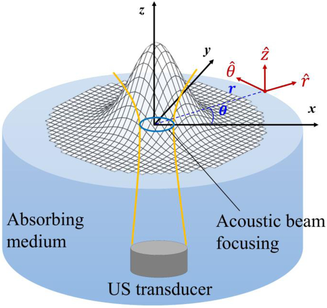
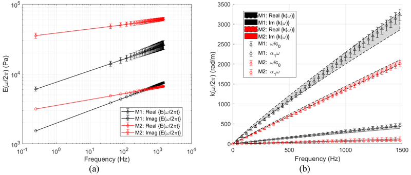
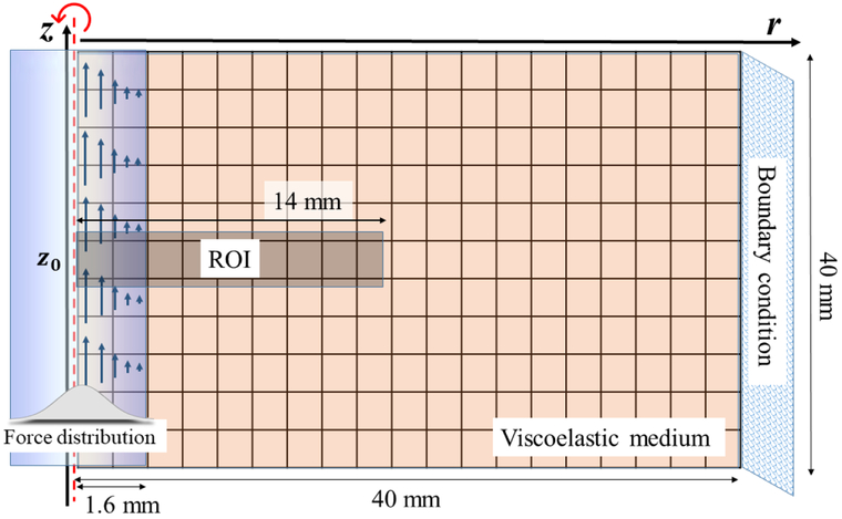
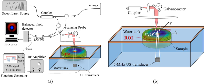
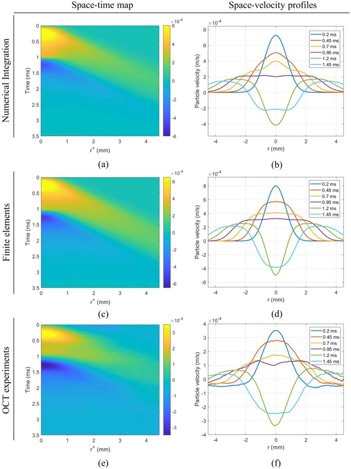
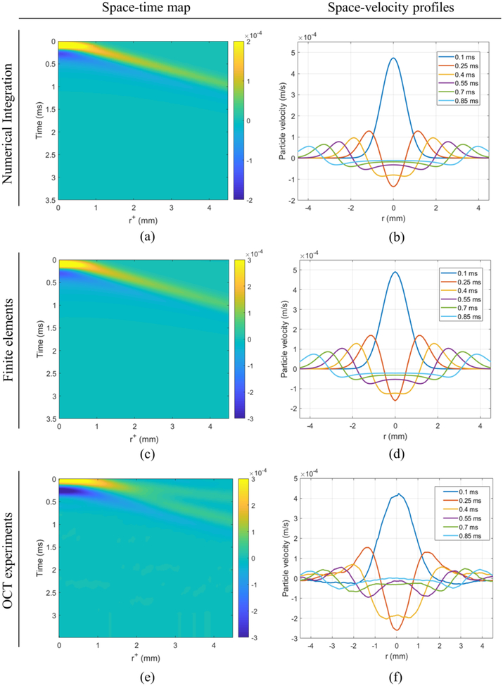
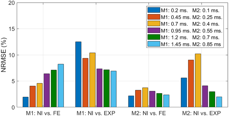
Many approaches to elastography incorporate shear waves; in some systems these are produced by acoustic radiation force (ARF) push pulses. Understanding the shape and decay of propagating shear waves in lossy tissues is key to obtaining accurate estimates of tissue properties, and so analytical models have been proposed. In this paper, we reconsider a previous analytical model with the goal of obtaining a computationally straightforward and efficient equation for the propagation of shear waves from a focal push pulse. Next, this model is compared with an experimental optical coherence tomography (OCT) system and with finite element models, in two viscoelastic materials that mimic tissue. We find that the three different cases-analytical model, finite element model, and experimental results-demonstrate reasonable agreement within the subtle differences present in their respective conditions. These results support the use of an efficient form of the Hankel transform for both lossless (elastic) and lossy (viscoelastic) media, and for both short (impulsive) and longer (extended) push pulses that can model a range of experimental conditions.

Figure 1.

Schematic of a Gaussian-shaped force pulse produced in a viscoelastic medium by an ultrasound ARF transducer. The center of the pulse is the origin of the coordinate systems, with r and θ as the radial and angular components in the cylindrical coordinate system, and x, y, and z as the Cartesian axes.

Figure 2.

Log-log of frequency-dependent complex Young’s modulus (a) and complex wave number (b) for both phantom materials M1 and M2, obtained from mechanical measurements using a stress relaxation by compression test. ω = 2πf, and f = frequency. Frequency-dependent results are predictions of the Kelvin-Voigt fractional derivative model and do not represent independent measurements over the frequency range.

Figure 3.

Schematic of a 2D finite element axisymmetric deformable part subjected to a Gaussian-shaped pulse in Abaqus/CAE version 6.14-1. Space-time representations of particle velocity ν_Z0 (r, t) were calculated in the region of interest (ROI).

Figure 4.

Experimental setup. (a) PhS-OCT system implemented with a swept-source laser for motion detection. (b) Placement of the phantom in a water tank, ARF US-transducer, and region of interest (ROI). Motion is produced close to the surface of the sample.

Figure 5.

Shear wave propagation in a medium material M1 in the form of space-time maps (left column), and space-velocity profiles for various time instants (right column). Motion is shown as particle velocity ν_z(r, t) for an input Gaussian body force of σ = 0.338 mm applied for a time duration of τ_M1 = 1ms. Color bars represent particle velocity in m/s. Legends in all plots (right column) correspond to time snapshot at six uniformly separated time instants.

Figure 6.

Shear wave propagation in a medium material M2 in the form of space-time maps (left column), and space-velocity profiles for various time instants (right column). Motion is shown as particle velocity ν_z (r, t) for a input Gaussian body force of σ = 0.338 mm applied for a time duration of τ_M1 = 0.1 ms. Color bars represent particle velocity in m/s. Legends in all plots (right column) correspond to time snapshot at six uniformly separated time instants.

Figure 7.

Quantitative comparison of numerical integration (NI) curves versus finite elements (FE) and OCT experiments (EXP) for each time instant and phantom material M1 and M2. Normalized root-mean-square error, shown as percentage, is used for the analysis of discrepancies between curves.

References

1. Abramowitz M, & Stegun IA (1965). Handbook of Mathematical Functions: With Formulas, Graphs, and Mathematical Tables: Dover Publications.
1. Baddour N (2011). Multidimensional wave field signal theory: Mathematical foundations. AIP Advances, 1(2), 022120.
1. Baddour N (2018). Addendum to foundations of multidimensional wave field signal theory: Gaussian source function. AIP Advances, 8(2), 025313.
1. Bercoff J, Tanter M, & Fink M (2004). Supersonic shear imaging: a new technique for soft tissue elasticity mapping. IEEE Transactions on Ultrasonics, Ferroelectrics, and Frequency Control, 51(4), 396–409. - PubMed
1. Blackstock DT (2000). Fundamentals of Physical Acoustics: Wiley.
Publication types