. 2018 Nov 20:9:1631.
doi: 10.3389/fphys.2018.01631. eCollection 2018.

Propulsive Power in Cross-Country Skiing: Application and Limitations of a Novel Wearable Sensor-Based Method During Roller Skiing

Affiliations

Propulsive Power in Cross-Country Skiing: Application and Limitations of a Novel Wearable Sensor-Based Method During Roller Skiing

Øyvind Gløersen et al. Front Physiol. .

Abstract

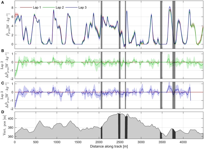
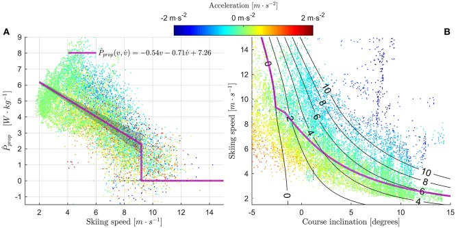
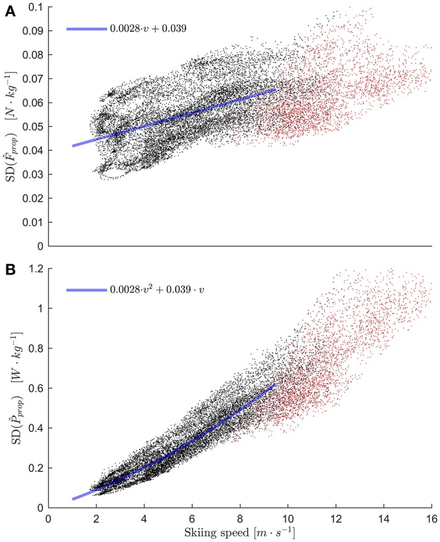
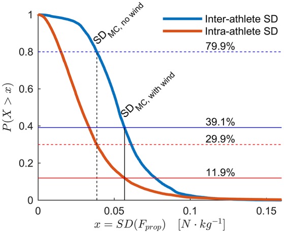
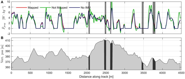
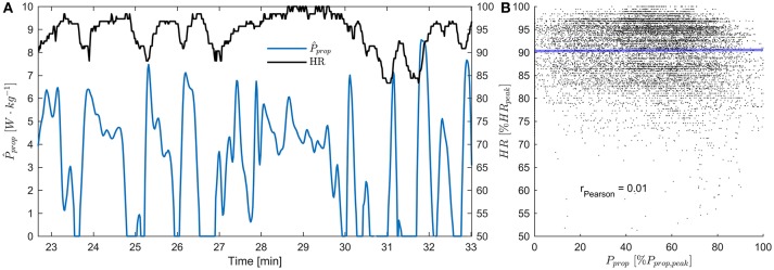
Cross-country skiing is an endurance sport that requires extremely high maximal aerobic power. Due to downhill sections where the athletes can recover, skiers must also have the ability to perform repeated efforts where metabolic power substantially exceeds maximal aerobic power. Since the duration of these supra-aerobic efforts is often in the order of seconds, heart rate, and pulmonary VO2 do not adequately reflect instantaneous metabolic power. Propulsive power (P prop) is an alternative parameter that can be used to estimate metabolic power, but the validity of such calculations during cross-country skiing has rarely been addressed. The aim of this study was therefore twofold: to develop a procedure using small non-intrusive sensors attached to the athlete for estimating P prop during roller-skiing and to evaluate its limits; and (2) to utilize this procedure to determine the P prop generated by high-level skiers during a simulated distance race. Eight elite male cross-country skiers simulated a 15 km individual distance race on roller skis using ski skating techniques on a course (13.5 km) similar to World Cup skiing courses. P prop was calculated using a combination of standalone and differential GNSS measurements and inertial measurement units. The method's measurement error was assessed using a Monte Carlo simulation, sampling from the most relevant sources of error. P prop decreased approximately linearly with skiing speed and acceleration, and was approximated by the equation P prop ( v , v ˙ ) = -0.54·v -0.71 · v ˙ + 7.26 W·kg-1. P prop was typically zero for skiing speeds >9 m·s-1, because the athletes transitioned to the tuck position. Peak P prop was 8.35 ± 0.63 W·kg-1 and was typically attained during the final lap in the last major ascent, while average P prop throughout the race was 3.35 ± 0.23 W·kg-1. The measurement error of P prop increased with skiing speed, from 0.09 W·kg-1 at 2.0 m·s-1 to 0.58 W·kg-1 at 9.0 m·s-1. In summary, this study is the first to provide continuous measurements of P prop for distance skiing, as well as the first to quantify the measurement error during roller skiing using the power balance principle. Therefore, these results provide novel insight into the pacing strategies employed by high-level skiers.

Keywords: GNSS; GPS; energy; force; validity; work rate.


Figures

Figure 1
Figure 1
Positioning of the two IMUs on the athletes' body and motivation for the frontal area model described in Equation 5. One IMU was positioned approximately at the level of the third thoracic vertebra, the other was taped laterally on the thigh approximately 10 cm inferior to the trochanter. The axes were aligned with the x-axis (blue) in the mediolateral direction and the y-axis (red) in the anterior direction. The z-axis (green) was aligned with gravity when the athletes were in a standing posture, as described in the text. The frontal areas of the torso and thighs scale approximately with the cosine of the pitch angles θ k = atan(ay, k/az, k), where ay, k and az, k are the smoothed accelerometer outputs along the y and z-axis respectively. k represents the thigh or torso location.
Figure 2
Figure 2
(A) Postures used to calculate frontal area. The first pose for each athlete was used to calculate the characteristic length L (Equation 3), which was defined as the width at the height of the pose's center of mass (green line). (B) Model for the frontal area A based on the postures in (A) and Equation 5. The data points are enumerated to match the postures in (A), and show the measurements from one subject. Red dots indicate measurements from all other subjects. (C) Model (Equations 7, 8) for the drag coefficient of a skier as a function of the Reynolds number (solid black line). Blue squares: data from Achenbach (1968); Green diamonds: data from van Ingen Schenau et al. (1982); Red circles: data from Spring et al. (1988); Dashed blue line: model fitted to Achenbach's measurements. The upper and lower x-axis were related by Equation 3 using atmospheric conditions as specified in van Ingen Schenau et al. (1982) and L = 0.3 m. Shaded areas indicate the models' standard deviations, and were obtained using Monte Carlo simulations (N = 5,000) sampled from the distributions specified in the statistics section.
Figure 3
Figure 3
Histogram of the squared magnitude of gyroscope measurements (angular velocity) during skiing for all athletes. The distinct distribution minimum at about 5,000°2s−2 indicates the transition from the tucked position, where movements of both torso and thigh are small, to skiing techniques that generate propulsion. In the current study, the athletes were assumed to be in the tucked position when |ω|2 of both torso and thigh were <5,000°2·s−2.
Figure 4
Figure 4
(A) Propulsive power normalized to body mass plotted over distance along the course for the three laps (lap 1 red, lap 2 green, lap 3 blue). Colored regions around the solid lines show the standard deviations from the Monte Carlo simulation. Vertical gray shading indicates regions where double differenced ambiguities were float. The Monte Carlo simulation does not account for the reduced accuracy in these regions. Negative values of Pprop occurs when Fprop < 0 and could be caused by either active breaking of the athlete, or by measurement error. (B) Mean difference in propulsive power between lap 2 and lap 1. Colored shaded region shows the 95% CI. (C) Same as B, but for the difference between lap 3 and lap 1. (D) Altitude profile of the competition course. Black regions correspond to the regions where double differenced ambiguities were float.
Figure 5
Figure 5
(A) Propulsive power (normalized to body mass) was approximately linearly related to skiing speed (v) and acceleration (v˙) in the skiing direction. Data from all athletes are included in the figure, and data points are color coded by v˙, as indicated by the colorbar above the figure. The magenta-colored line is the least squares regression fit to samples where the athlete was not in the tucked position. The shaded region indicates the measurement error (SD), see Figure 7 for details. (B) Plot of skiing speed vs. the course inclination. Data points are color coded as in panel (A). The black lines indicate constant propulsive power (in W·kg−1), assuming constant skiing speed (v˙ = 0). The magenta line shows the steady state skiing speed obtained from the regression line in (A). It was defined as the real root of the 3rd degree polynomial obtained by replacing Pprop with Pprop(v,v˙) in Equation 1, and assuming a constant drag area of 0.55 m2 and average body mass 77.1 kg. For v > 9 m·s−1 the line was defined to follow the zero-Pprop iso-line. The figure clearly shows that data points where v˙ ≈ 0 (green color) are distributed close to the steady-state speed line, as expected. Data points below the steady-state line have v˙ > 0 (red), and data points above the line have v˙ < 0. This is mainly attributed to the athletes' inertias.
Figure 6
Figure 6
(A) Frontal areas (Â) estimated from the accelerometer outputs plotted over skiing speed, normalized by body mass (using an allometric scaling coefficient of 2/3). Red dots represent measurements where the skiers were in the tucked position. Blue line: logistic function fitted to the data (Equation 6). Athletes typically assumed the tucked position at skiing speeds >9.1 m·s−1. (B) Drag areas normalized to body mass (·CD) found in the current study plotted over skiing speed for all athletes. The blue line shows the product of the frontal area model from Equation 6 (plotted in panel A) and the drag coefficient (Equation 8, Figure 2). Models used by Sundström et al. (2013), Moxnes et al. (2014), and Swarén and Eriksson (2017) are included for comparison.
Figure 7
Figure 7
(A) Standard deviation of propulsive force (normalized to body mass) calculated from the Monte Carlo simulation plotted over skiing speed. The red dots are measurements when the athletes were in the tucked position. In a later step propulsive power (and force) was defined to be zero for these samples, but they are included in this figure to illustrative purposes. The blue line is the least squares linear regression line fitted to the data points where the athletes were not in the tucked position. (B) same as (A), but for Pprop. Since Pprop = Fprop·v, the regression line from (A) multiplied with v fits well to the data.
Figure 8
Figure 8
In order to discriminate the Fprop or Pprop generated by high-level athletes, the methods accuracy must be better than typical athlete-to-athlete or within-athlete differences. To that end, this figure displays the empirical complementary cumulative distribution function (ECCDF) of typical athlete-to-athlete differences in Fprop measured at the same position along the course (blue line). More specifically, it shows the between-athlete standard deviation of Fprop evaluated at every integer meter along the course, excluding measurements where the athletes were in the tucked position. The red line is the ECCDF of the within-athlete lap-to-lap standard deviation. The solid vertical line at 0.0568 N·kg−1 shows the mean standard deviation of Fprop from the Monte Carlo simulation, which reflects the methods typical accuracy under the specified conditions. For comparison, the dotted vertical line at 0.0385 N·kg−1 shows the mean standard deviation of Fprop from another Monte Carlo simulation assuming zero-wind conditions. With the measured wind conditions, inter-athlete SD was greater than the typical measurement accuracy only for 39.1% of the course, and intra-athlete SD only for 11.9% of the course. Under the zero-wind assumption, the inter- and intra-athlete differences were greater than the measurement accuracy for 79.9 and 29.9% of the course, respectively.
Figure 9
Figure 9
(A) Comparison of propulsive power calculations using mapping on dGNSS reference (blue line), calculations using only measurements from the standalone GNSS receiver (green line), and using the simplified drag area model based on body mass and skiing speed (Equation 6, red line). Data are from one lap for a single athlete. Vertical gray shading indicates regions where double differenced ambiguities were float. (B) Altitude profile of the competition course. Black regions correspond to the regions where double difference ambiguities were float.
Figure 10
Figure 10
(A) Heart rate (HR) and Pprop measurements during the third lap for an example athlete. HR is expressed relative to the peak HR measured during the test race. (B) Scatter plot showing all measurements of Pprop (normalized to each athlete's peak Pprop) vs. all measurements of HR. There was no significant correlation between the two parameters (rPearson = 0.01, p = 0.18). This indicates that changes in Pprop during cross-country ski races are too fast for heart rate to provide a valid measure of instantaneous metabolic power.

References

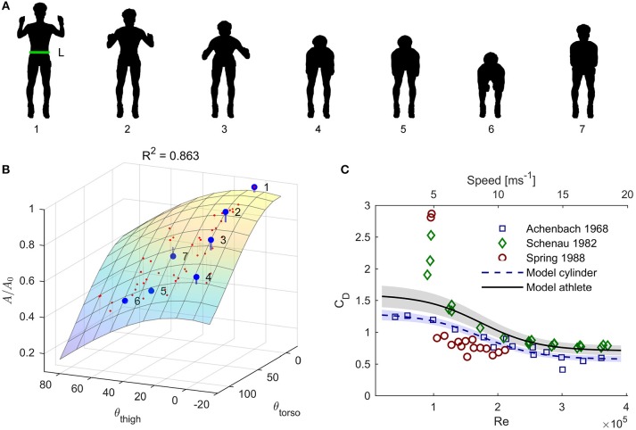
    1. Achenbach E. (1968). Distribution of local pressure and skin friction around a circular cylinder in cross-flow up to Re = 5*106. J. Fluid Mech 34, 625–639. 10.1017/S0022112068002120 - DOI
    1. Ainegren M., Carlsson P., Tinnsten M. (2008). Rolling resistance for treadmill roller skiing. Sport. Eng. 11, 23–29. 10.1007/s12283-008-0004-1 - DOI
    1. Aleshinsky S. Y. (1986). An energy ‘sources' and ‘fractions' approach to the mechanical energy expenditure problem. J. Biomech. 19, 287–315. - PubMed
    1. Andersson E., Björklund G., Holmberg H.-C., Ørtenblad N. (2017). Energy system contributions and determinants of performance in sprint cross-country skiing. Scand. J. Med. Sci. Sports 27, 385–398. 10.1111/sms.12666 - DOI - PubMed
    1. Andersson E., Supej M., Sandbakk Ø., Sperlich B., Stoggl T., Holmberg H. C. (2010). Analysis of sprint cross-country skiing using a differential global navigation satellite system. Eur. J. Appl. Physiol. 110, 585–595. 10.1007/s00421-010-1535-2 - DOI - PubMed