Deep convolutional networks do not classify based on global object shape

Abstract

Deep convolutional networks (DCNNs) are achieving previously unseen performance in object classification, raising questions about whether DCNNs operate similarly to human vision. In biological vision, shape is arguably the most important cue for recognition. We tested the role of shape information in DCNNs trained to recognize objects. In Experiment 1, we presented a trained DCNN with object silhouettes that preserved overall shape but were filled with surface texture taken from other objects. Shape cues appeared to play some role in the classification of artifacts, but little or none for animals. In Experiments 2-4, DCNNs showed no ability to classify glass figurines or outlines but correctly classified some silhouettes. Aspects of these results led us to hypothesize that DCNNs do not distinguish object's bounding contours from other edges, and that DCNNs access some local shape features, but not global shape. In Experiment 5, we tested this hypothesis with displays that preserved local features but disrupted global shape, and vice versa. With disrupted global shape, which reduced human accuracy to 28%, DCNNs gave the same classification labels as with ordinary shapes. Conversely, local contour changes eliminated accurate DCNN classification but caused no difficulty for human observers. These results provide evidence that DCNNs have access to some local shape information in the form of local edge relations, but they have no access to global object shapes.

Fig 1. Demonstration of the importance of global shape in object recognition.

(a) Silhouette of a bear; (b) Scrambled natural image of a bear (See text). Image URLs are in S2 File.

Fig 2. Sample stimuli used in Experiment 1.

The bounding shape of an object was combined with the texture of a different object to generate each image. a) Shape: Teapot | Texture: Golf ball; b) Shape: Vase | Texture: Gong; c) Shape: Airplane | Texture: Otter; d) Shape: Obelisk | Texture: Lobster; e) Shape: Cannon | Texture: Pineapple; f) Shape: Ram | Texture: Bison; g) Shape: Camel | Texture: Zebra; h) Shape: Orca | Texture: Kimono; i) Shape: Otter | Texture: Speedometer; j) Shape: Elephant | Texture: Sock. The full image set is displayed in Figs 3–6.

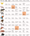
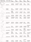
Fig 3. Network classifications for the stimuli presented in Experiment 1 Part 1.

The left most column shows the image presented. The second column in each row names the object from which the shape was sampled. The third column names the object from which the texture silhouette was obtained. Probabilities assigned to the object name in columns 2 and 3 are shown as percents below the object label. The remaining five columns show the probabilities (as percents) produced by the network for its top five classifications, ordered left to right in terms of probability. Correct shape classifications in the top five are shaded in blue and correct texture classifications are shaded in orange.

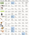
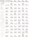
Fig 4. Network classifications for the stimuli presented in Experiment 1 Part 2.

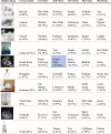
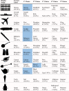
Fig 5. Network classifications for the stimuli presented in Experiment 1 Part 3.

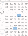
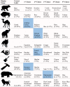
Fig 6. Network classifications for the stimuli presented in Experiment 1 Part 4.

Fig 7. Comparison of probabilities assigned to image shapes and textures for animals.

On the x-axis, the shape and texture of each object are given as shape-texture. Filled black bars display the probability given by the network to the correct shape. Outlined bars display the probability given by the network for the correct texture.

Fig 8. Comparison of probabilities assigned to image shapes and textures for artifacts.

On the x-axis, the shape and texture of each object are given as shape-texture. Filled black bars display the probability given by the network to the correct shape. Outlined bars display the probability given by the network for the correct texture.

Fig 9. Sample stimuli used in Experiment 2.

Fig 10. VGG-19 classifications for glass figurines Part 1.

The leftmost column shows the image presented to the VGG-19 DCNN. The second column shows the correct object label and the probability generated by the network for that label. The other five columns show probabilities for the network’s top five classifications, ordered left to right from highest to lowest. Correct classifications are shaded in blue.

Fig 11. VGG-19 classifications for glass figurines Part 2.

Fig 12. Five additional glass Pianos.

VGG-19 incorrectly classified each of these five images despite correctly classifying the glass piano shown in Fig 11.

Fig 13. Sample outline stimuli used in Experiment 3.

Fig 14. VGG-19 classifications for object outlines Part 1.

The leftmost column is the image presented to the DCNN. The second column from the left is the correct object label and the classification probability produced for that label. The other five columns show probabilities for the VGG-19’s top five classifications, ordered left to right in terms of the probability given by the network. Correct classifications are shaded in blue.

Fig 15. VGG-19 classifications for object outlines Part 2.

Fig 16. VGG-19 classifications for object outlines Part 3.

Fig 17. VGG-19 classifications for object outlines Part 4.

Fig 18. Sample stimuli used in Experiment 4.

Fig 19. VGG-19 classifications for black object silhouettes Part 1.

The leftmost column shows the image presented to VGG-19. The second column from the left shows the correct object label and the classification probability produced for that label. The other five columns show probabilities for the network’s top five classifications, ordered left to right in terms of the probability given by the network. Correct classifications are shaded in blue.

Fig 20. VGG-19 classifications for black object silhouettes Part 2.

Fig 21. VGG-19 classifications for black object silhouettes Part 3.

Fig 22. VGG-19 classifications for black object silhouettes Part 4.

Fig 23. Stimuli used in Experiment 5a.

Top row: the original silhouette images, all correctly classified by VGG-19 (appearing in top-five). Bottom row: Scrambled images on which the network was tested.

Fig 24. VGG-19 classifications for part-scrambled silhouettes.

The leftmost column shows the image presented to the DCNN. The second column shows the correct object label and the classification probability produced by the network for that label. The other five columns show probabilities for the network’s top five classifications, ordered left to right from highest to lowest. Correct classifications are shaded in blue.

Fig 25. VGG-19 for unscrambled and part-scrambled images.

Bars show probabilities for correct responses for each of the objects. Probability is plotted on a logarithmic scale to make small values visible.

Fig 26. Stimuli used in Experiment 5b.

Top row: the original silhouette images, all correctly classified by the network. Bottom row: images with local contour features disrupted.

Fig 27. VGG-19 classifications for serrated edge silhouettes.

The leftmost column shows the image presented to the DCNN. The second column shows the correct object label and the classification probability produced by the network for that label. The other five columns show probabilities for the network’s top five classifications, ordered left to right from highest to lowest. Correct classifications are shaded in blue.

Fig 28. Comparison of VGG-19 performance for locally perturbed contours with unscrambled and part-scrambled images.

Bars show probabilities for correct responses for each of the objects. Probability is plotted on a logarithmic scale to make small values visible.

References

1. Yampolskiy R. Turing test as a defining feature of AI-completeness. Artificial Intelligence, Evolutionary Computing and Metaheuristics. 2013:3–17.
1. Turing AM. Computing machinery and intelligence. Mind. 1950. October 1;59(236):433–60.
1. Geman D, Geman S, Hallonquist N, Younes L. Visual turing test for computer vision systems. Proceedings of the National Academy of Sciences. 2015. March 24;112(12):3618–23. - PMC - PubMed
1. Krizhevsky A, Sutskever I, Hinton GE. Imagenet classification with deep convolutional neural networks. In: Advances in Neural Information Processing Systems, 2012. (pp. 1097–1105).
1. Gunji N, Higuchi T, Yasumoto K, Muraoka H, Ushiku Y, Harada T, Kuniyoshi Y. Scalable multiclass object categorization with Fisher based features. ILSVRC 2012, The Univ. of Tokyo.
Publication types