A nearest-neighbors network model for sequence data reveals new insight into genotype distribution of a pathogen

Abstract

Background: Sequence similarity networks are useful for classifying and characterizing biologically important proteins. Threshold-based approaches to similarity network construction using exact distance measures are prohibitively slow to compute and rely on the difficult task of selecting an appropriate threshold, while similarity networks based on approximate distance calculations compromise useful structural information.

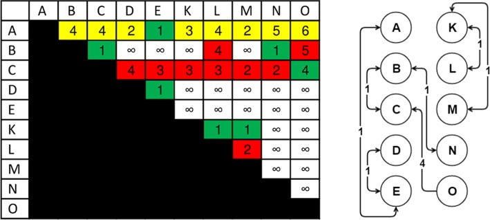
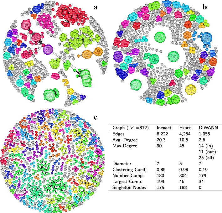
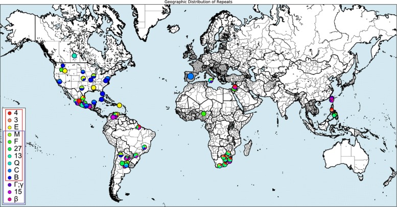
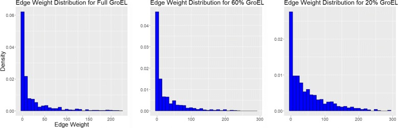
Results: We present an alternative network representation for a set of sequence data that overcomes these drawbacks. In our model, called the Directed Weighted All Nearest Neighbors (DiWANN) network, each sequence is represented by a node and is connected via a directed edge to only the closest sequence, or sequences in the case of ties, in the dataset. Our contributions span several aspects. Specifically, we: (i) Apply an all nearest neighbors network model to protein sequence data from three different applications and examine the structural properties of the networks; (ii) Compare the model against threshold-based networks to validate their semantic equivalence, and demonstrate the relative advantages the model offers; (iii) Demonstrate the model's resilience to missing sequences; and (iv) Develop an efficient algorithm for constructing a DiWANN network from a set of sequences. We find that the DiWANN network representation attains similar semantic properties to threshold-based graphs, while avoiding weaknesses of both high and low threshold graphs. Additionally, we find that approximate distance networks, using BLAST bitscores in place of exact edit distances, can cause significant loss of structural information. We show that the proposed DiWANN network construction algorithm provides a fourfold speedup over a standard threshold based approach to network construction. We also identify a relationship between the centrality of a sequence in a similarity network of an Anaplasma marginale short sequence repeat dataset and how broadly that sequence is dispersed geographically.

Conclusion: We demonstrate that using approximate distance measures to rapidly construct similarity networks may lead to significant deficiencies in the structure of that network in terms centrality and clustering analyses. We present a new network representation that maintains the structural semantics of threshold-based networks while increasing connectedness, and an algorithm for constructing the network using exact distance measures in a fraction of the time it would take to build a threshold-based equivalent.

Keywords: Anaplasma marginale Msp1a; Centrality; Clustering; GroEL; Network analysis; Sequence similarity network.

Fig. 1

An example showing how DiWANN nodes connect. The example has four nodes, A–D, corresponding to sequences. Weights along the lines show absolute edit distances. Solid lines indicate edges that would be present in the DiWANN graph, while dotted lines show relationships where there would be no edges. The DiWANN graph is structurally different from any threshold-based distance graph

Fig. 2

An example illustrating the workings of the DiWANN network construction algorithm. To the left is the distance matrix produced by Algorithm 1, and to the right is the DiWANN graph constructed using this distance matrix. The example has 10 sequences drawn from the A. marginale SSRs. Because the distance matrix is symmetric, Algorithm 1 uses only its upper diagonal half, while the unused portion is in black. The first row of the matrix, which must always be computed, is shown in yellow. Every cell in which a distance is computed but is not used in building the DiWANN graph is shown in red. A cell in which a distance is pruned because it wouldn’t result in an edge in the DiWANN graph is shown with entry of infinity. All other non-infinite cell values, shown in green, correspond to edges in the graph. For each sequence, A-O, an outgoing edge is added to the sequence (sequences) that is (are) at the minimum distance from itself (corresponds to rowMin at the end of a row computation in Algorithm 1). Note that the edge from node O is not bidirectional

Fig. 3

A. marginale sequence similarity networks. Subplot a shows the inexact similarity network at a 6% difference threshold. Subplot b shows an exact distance network at threshold 2. Subplot c shows the DiWANN network. All three graphs are for the A. marginale SSR data set

Fig. 4

Degree distributions of A. marginale sequence similarity networks. This figure shows the degree distributions for each of the SSNs shown in Fig. 3. Subplot a shows the degrees of the inexact similarity network at a 6% difference threshold. Subplot b shows degrees of the an exact distance network at threshold 2. Subplot c shows degrees (combined in and out degree) of the DiWANN network. All three graphs are for the A. marginale SSR data set

Fig. 5

A. marginale sequence similarity networks with the most central nodes highlighted. Each figure has been modified to size nodes by their PageRank centrality. The ten most central nodes are highlighted in red. Subplot a shows the inexact similarity network at a 6% difference threshold. Subplot b shows an exact distance network at threshold 2. Subplot c shows the DiWANN network. All three graphs are for the A. marginale SSR data set

Fig. 6

A. marginale sequence similarity networks. Subplots a-c show the inexact (Blast similarity score > 95%), exact (distance ≤ 2) and DiWANN networks for the A. marginale SSR data, respectively. The table gives some structural properties for each of these networks. Nodes are sized based on their PageRank centrality, and colored based on their cluster membership using the Louvain community detection algorithm

Fig. 7

GroEL sequence similarity networks. Subplots a-c show the inexact (Blast similarity score > 75%), exact (distance ≤ 30) and DiWANN networks, respectively, for the GroEL data. The table gives some structural properties for each of these networks. Nodes are sized based on their PageRank centrality, and colored based on their cluster membership using the Louvain community detection algorithm

Fig. 8

Gold standard sequence similarity networks. Subplots a-c show the inexact (Blast similarity score > 55%), exact (distance ≤ 150) and DiWANN networks, respectively, for the gold standard data. The table gives some structural properties for each of these networks. Nodes are sized based on their PageRank centrality, and colored based on their cluster membership using the Louvain community dtection algorithm

Fig. 9

A map of the 10 most common and 10 most central A. marginale Msp1a SSRs. This map, generated by RepeatAnalyzer, shows the distribution of the 10 SSRs which appear across the greatest number of countries, as well as those which are most central in the graph representation of the data. In the legend, central SSRs are in the red box, while common SSRs are in the blue box

Fig. 10

Alignment and logos of the most common and most central SSRs. Panel a of this figure shows the alignment for the ten most common (geographically) and ten most central (in the DiWANN network) A. marginale SSRs. The top three entries are SSRs which are only common, while the bottom 3 are only central. Those in the middle seven rows belong to both sets. The logo in panel b represents the most central SSRs, while the one in panel c represents the most common SSRs

Fig. 11

Edge weight distributions for the GroEL dataset. These plots show the distribution of edge weights in the DiWANN networks using the full GroEL data, averages for five 60% samples and averages for five 20% samples. The minimum edge weight for all three networks is 1. For the 20% networks, the median is 4 and the maximum is 223. For the 60% networks, the median is 6 and the maximum is 288. For the full network, the median is 29 and the maximum is 291