Coherent chaos in a recurrent neural network with structured connectivity

Abstract

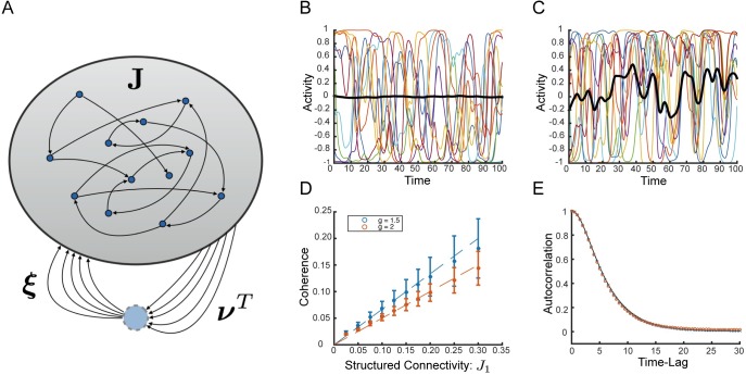
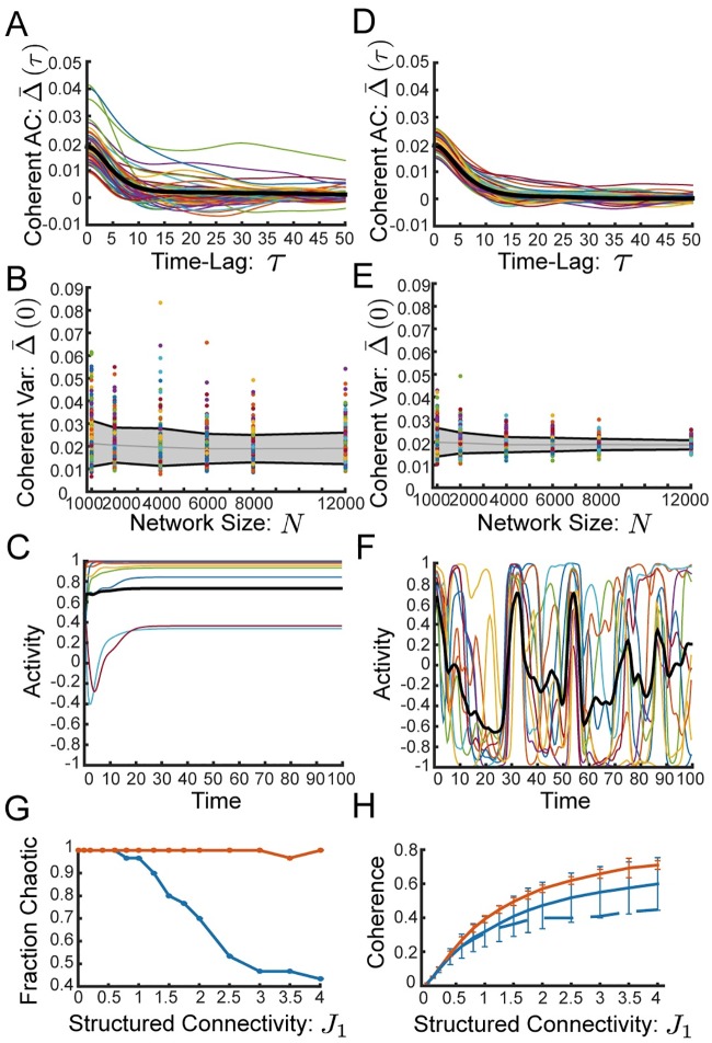
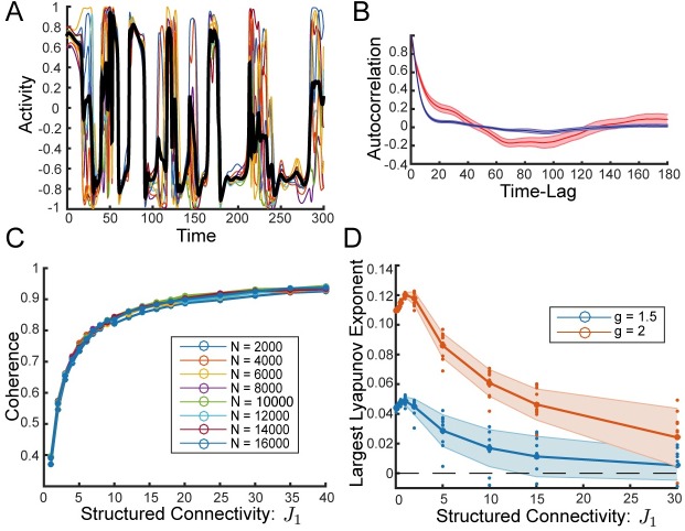
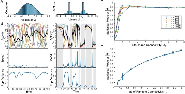
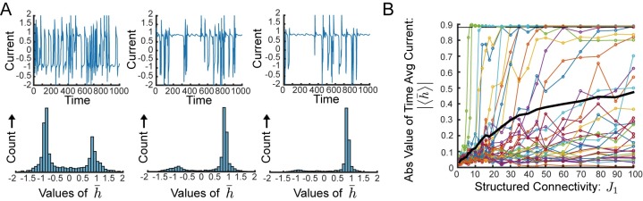
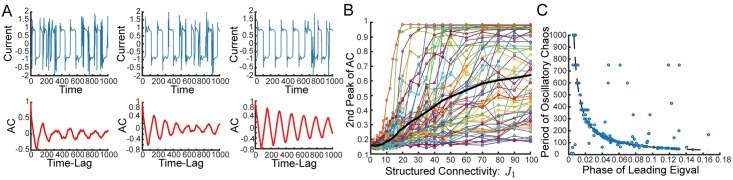
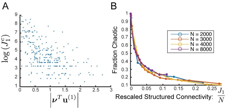
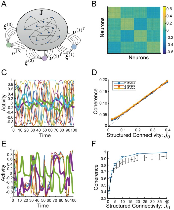
We present a simple model for coherent, spatially correlated chaos in a recurrent neural network. Networks of randomly connected neurons exhibit chaotic fluctuations and have been studied as a model for capturing the temporal variability of cortical activity. The dynamics generated by such networks, however, are spatially uncorrelated and do not generate coherent fluctuations, which are commonly observed across spatial scales of the neocortex. In our model we introduce a structured component of connectivity, in addition to random connections, which effectively embeds a feedforward structure via unidirectional coupling between a pair of orthogonal modes. Local fluctuations driven by the random connectivity are summed by an output mode and drive coherent activity along an input mode. The orthogonality between input and output mode preserves chaotic fluctuations by preventing feedback loops. In the regime of weak structured connectivity we apply a perturbative approach to solve the dynamic mean-field equations, showing that in this regime coherent fluctuations are driven passively by the chaos of local residual fluctuations. When we introduce a row balance constraint on the random connectivity, stronger structured connectivity puts the network in a distinct dynamical regime of self-tuned coherent chaos. In this regime the coherent component of the dynamics self-adjusts intermittently to yield periods of slow, highly coherent chaos. The dynamics display longer time-scales and switching-like activity. We show how in this regime the dynamics depend qualitatively on the particular realization of the connectivity matrix: a complex leading eigenvalue can yield coherent oscillatory chaos while a real leading eigenvalue can yield chaos with broken symmetry. The level of coherence grows with increasing strength of structured connectivity until the dynamics are almost entirely constrained to a single spatial mode. We examine the effects of network-size scaling and show that these results are not finite-size effects. Finally, we show that in the regime of weak structured connectivity, coherent chaos emerges also for a generalized structured connectivity with multiple input-output modes.

Fig 1. Random network with structured connectivity generates coherent chaos.

(A) Network schematic showing neurons connected via random matrix J and rank-one structured connectivity. The structured component is represented schematically as a loop with drive through the output mode, ν, and feedback through the input mode, ξ. In our model these two vectors are orthogonal. The standard deviation of the random component is given by $\frac{g}{\sqrt{N}}$ and the strength of the structured component is $\frac{J_1}{\sqrt{N}}$. (B) Sample network dynamics without structured component, i.e. J₁ = 0. Colored traces show a random collection of ten neural activity patterns, ϕ_j, black trace shows the coherent mode activity, $\overline{\varphi }=\frac{1}{N}{\mathit{\xi }}^T\varphi$, which exhibits only miniscule fluctuations. (C) Sample dynamics for J₁ = 1. Coherent mode displays substantial fluctuations. (D) Coherence, χ (definition in text), as a function of the strength of structured connectivity component, J₁ for small values of J₁. Simulation and theory (valid in the weak structured connectivity regime—J₁ ≪ g) shown for both g = 1.5 and g = 2. Bars show standard deviation over 60 realization of the random connectivity. (E) Passive coherent chaos. With weak structured connectivity fluctuations of the coherent mode follow the fluctuations of the independent residual components. Normalized autocorrelation of the coherent component of the current, $\overline{q}\left(\tau \right)$, in red circles. Average normalized autocorrelation of the residuals, q_δ(τ), in blue ‘x’s. Both are averaged over 60 realizations of the random connectivity with J₁ = 0.1. Prediction from theory in black. N = 4000 and g = 2 in all panels unless stated otherwise.

Fig 2. Row balance preserves chaos, and increases coherence.

(A) Full coherent mode autocorrelation, $\overline{\Delta }\left(\tau \right)$ of 60 individual realizations. Thick black line shows average over realizations. Network with random connectivity J without row balance exhibits significant difference between realizations. (B) Coherent mode variance, $\overline{\Delta }\left(0\right)$, as a function of network size for 300 individual realizations. Gray line shows average and gray region with black boundary shows one standard deviation over realizations. Without row balance the standard deviation (over realizations) saturates to a finite value as the network size increases, indicating that the variability between realizations is not a finite-size effect. (C) Without row balance a network with moderate structured connectivity (J₁ = 2.5) exhibits a fixed point. (D)-(F) Same as (A)-(C) respectively, but network has “row balance” random connectivity, $\tilde{\mathbf{J}}=\mathbf{J}-\mathbf{J}\frac{\mathit{\xi }{\mathit{\xi }}^T}{N}$. (D) Individual realizations of Δ(τ) are all very close to the average. (E) With row balance the standard deviation of Δ(0) over realizations shrinks with N, suggesting that the variability between realizations is a finite-size effect. (F) Same realization of J as in (C), but with row balance. Chaos is preserved. (G)-(H) Networks without row balance in blue, with row balance in red (G) Fraction of realizations (out of 30 realizations) that lead to chaotic dynamics, as a function of structural connectivity, J₁. Row balance keeps nearly all realizations chaotic. (H) Coherence, χ, as a function of J₁ computed for the realizations from (E). Row balance increases coherence. Error bars display standard deviation. Full line shows all realizations, dashed line displays average coherence restricted to the chaotic realizations. J₁ = 0.2, g = 2, and N = 4000 for all panels unless otherwise noted.

Fig 3. Strong structured connectivity with row balance generates high coherence even as chaos persists.

(A) Sample activity of 10 randomly chosen neurons, ϕ_j, and coherent mode activity, $\overline{\varphi }$, in black. Strong structured connectivity with row balance subtraction to the random component of connectivity yields chaotic activity that is highly coherent with switching-like behavior. (B) Normalized autocorrelation of coherent mode, $\overline{q}\left(\tau \right)$, in red. Average normalized autocorrelation of the residuals, q_δ (τ), in blue. Shaded regions show standard deviation over 25 initial conditions of the same connectivity. Strong structured connectivity yields coherent mode dynamics that are qualitatively different from those of the residuals. J₁ = 15.8 for both (A) and (B), compare to Fig 1C and 1E, respectively. (C) Coherence, χ, as a function of J₁ is independent of network size. Coherence appears to approach 1 as J₁ is increased demonstrating that chaos persists even as fluctuations in the residuals shrink (See also S4 Fig). Coherence is averaged over 30 realizations of the connectivity for each N, excluding the few fixed points and limit cycles that occur for larger J₁ (2 out of 30 or less for the largest values of N). (D) Largest Lyapunov exponent as a function of J₁. Thick line shows average over 10 realizations, small dots show values for individual realizations, and shaded region is standard deviation. All but a small fraction of realizations are chaotic, even in the region where χ > 0.9. N = 4000 and g = 2 in all panels unless noted otherwise.

Fig 4. Self-tuned coherent chaos.

(A)-(B) Comparison between weak structured connectivity (Left: J₁ = 0.8) and stronger structured connectivity (Right: J₁ = 15.8) Both with N = 4000. (A) Histogram of values of the coherent mode current, $\overline{h}\left(t\right)$. Mild structured connectivity yields coherent fluctuations with a peak at zero and a distribution that appears not far from Gaussian. For stronger structured connectivity the histogram is clearly non-Gaussian and highly bimodal. (B) Top: Sample activity of 10 randomly chosen neurons, ϕ_i (t) and coherent mode activity, $\overline{\varphi }\left(t\right)$. Middle: Speed of network during same epoch of activity, (definition in text). Bottom: Instantaneous population variance of the residual currents δh_i (t). For mild structured connectivity, $\overline{\varphi }\left(t\right)$ fluctuates around zero (top), speed is roughly constant throughout the trial (middle), residual currents maintain large variance throughout (bottom). On the other hand, for stronger structured connectivity, there is state-switching between bouts of high and low coherent-mode activity (top), these same bouts are associated with vanishing speed (middle), and with small residual currents (bottom). Gray shaded regions show epochs of speed lower than 0.18, which was the lowest instantaneous speed achieved without structured connectivity. (C) Statistical mode (most frequent value) of $\mid \overline{h}\mid$ as a function of J₁. The results indicate a crossover to self-tuned coherent chaos, defined by the bimodal peaks of $\mid \overline{h}\mid$ reaching a constant value. The crossover occurs very rapidly and independently of N. Dashed line shows ${\overline{h}}^c={\varphi }^{\prime -1}\left(\frac{1}{g}\right)$. (D) The statistical mode of $\mid \overline{h}\mid$ as a function of g with fixed J₁ = 10 and N = 8000. Dashed line shows ${\overline{h}}^c={\varphi }^{\prime -1}\left(\frac{1}{g}\right)$. In all other panels g = 2.

Fig 5. Realization-dependent symmetry breaking in the self-tuned chaotic regime.

(A) Sample traces of coherent mode current, $\overline{h}\left(t\right)$, (top) and histogram of values of $\overline{h}\left(t\right)$ (bottom) from a connectivity realization with real eigenvalue for J₁ = 40,60,80 increasing from left to right. Dynamics exhibit pronounced asymmetry. (B) Absolute value of the time-average coherent mode current, $\mid \langle \overline{h}\rangle \mid$, as a function of J₁. Each colored line represents a single connectivity realization, averaged over 10 initial conditions. For many individual realizations, $\mid \langle \overline{h}\rangle \mid$ is significantly non-zero over a large range of values of J₁, while still not arriving at fixed point value (displayed by dashed line). We display the 37 realizations with real leading eigenvalue out of 100 total realizations from this set of trials. Thick black line shows average over those realizations. Dashed line shows ${\overline{h}}^c={\varphi }^{\prime -1}\left(\frac{1}{g}\right)$. N = 8000 for all panels.

Fig 6. Realization-dependent oscillatory imprint on the self-tuned chaotic regime.

(A) Sample traces $\overline{h}\left(t\right)$ (top), and normalized autocorrelation $\overline{q}\left(\tau \right)$ (bottom) of coherent mode current for a connectivity realization with complex eigenvalue for J₁ = 25,30,35 increasing from left to right. Dynamics exhibit pronounced oscillatory power and the autocorrelation exhibits a pronounced peak near the same frequency that will dominate the limit cycle for larger J₁. (B) Height of second peak of the autocorrelation of the coherent mode input as a function of J₁. Each colored line represents a single connectivity realization, averaged over 10 initial conditions. For many realizations, there is a significant second peak in the autocorrelation over a long range of values of J₁ well before a limit cycle is reached. We display the 63 realizations which had complex leading eigenvalue out of 100 in this set of trials. Thick black line shows average over those realizations. (C) Observed period of oscillatory chaos vs phase of leading eigenvalue for 181 realizations from which we were able to measure an oscillatory period with chaotic fluctuations (out of 196 realizations with complex leading eigenvalue in this set of trials. In order to confine to realizations and values of J₁ that yielded chaos, we restrict to those with second peak of autocorrelation less than 0.8. These had average height of second peak over all realizations: 0.5). Dotted line shows prediction from theory: $\frac{2\pi }{\text{Phase}\left({\lambda }_1\right)}$. The bulk of realizations are very well predicted although a notable fraction are not. The median error of prediction was 7.75 (average period over these realizations: 231, std: 212). N = 8000 for all panels.

Fig 7. Sufficiently strong structure yields transition out of chaos despite row balance.

(A) Scatterplot of the logarithm of transitional value, $J_1^c$, vs the absolute value of the projection of the output mode, ν, on the leading eigenvector, u⁽¹⁾ for 300 connectivity realizations with N = 8000. r² = 0.29. (B) Fraction of realizations displaying chaotic activity as a function of the rescaled structured connectivity: $\frac{J_1}{N}$. With this scaling the curve appears to be independent of N.

Fig 8. Coherent chaos along multiple modes.

(A) Schematic of network with three coherent modes displaying effective output modes, ν^(k), and input modes, ξ^(k), each of which are orthogonal to all others. (B) Matrix of Pearson correlation coefficients between firing rates, ϕ_i, of pairs of neurons in a network with three coherent modes and J₁ = 1. (C) Sample activity trace displaying sample single neuron activities and in thicker lines, three coherent mode activities, ${\overline{\varphi }}^{\left(k\right)}$. (D) Generalized coherence, χ^(k), as a function of J₁ for 2,3,4 modes in the regime of passive coherence. Dashed line displays theory. (E) Sample activity traces display extreme coherence for two coherent modes. (F) Generalized coherence for two coherent modes with row balance random connectivity (in blue) as a function of J₁ extends to near complete coherence, while chaos persists. Compare network with one coherent mode (in black dashed line). Bar shows standard deviation over 100 realizations. For panels (B), (C), (E) N = 2000. For panels (D) and (F) N = 4096.

References

1. Softky WR, Koch C. The highly irregular firing of cortical cells is inconsistent with temporal integration of random EPSPs. The Journal of neuroscience: the official journal of the Society for Neuroscience. 1993;13(1):334–50. 10.1523/JNEUROSCI.13-01-00334.1993 - DOI - PMC - PubMed
1. Churchland AK, Kiani R, Chaudhuri R, Wang XJ, Pouget A, Shadlen MN. Variance as a Signature of Neural Computations during Decision Making. Neuron. 2011;69(4):818–831. 10.1016/j.neuron.2010.12.037 - DOI - PMC - PubMed
1. Volgushev M, Chauvette S, Timofeev I. Long-range correlation of the membrane potential in neocortical neurons during slow oscillation. Progress in Brain Research. 2011;193:181–199. 10.1016/B978-0-444-53839-0.00012-0 - DOI - PMC - PubMed
1. Smith Ma, Kohn A. Spatial and temporal scales of neuronal correlation in primary visual cortex. The Journal of neuroscience: the official journal of the Society for Neuroscience. 2008;28(48):12591–603. 10.1523/JNEUROSCI.2929-08.2008 - DOI - PMC - PubMed
1. Cohen MR, Maunsell JHR. Attention improves performance primarily by reducing interneuronal correlations. Nature Neuroscience. 2009;12(12):1594–1600. 10.1038/nn.2439 - DOI - PMC - PubMed
Publication types