Flexible Coupling in Joint Inversions: A Bayesian Structure Decoupling Algorithm

Abstract

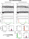
When different geophysical observables are sensitive to the same volume, it is possible to invert them simultaneously to jointly constrain different physical properties. The question addressed in this study is to determine which structures (e.g., interfaces) are common to different properties and which ones are separated. We present an algorithm for resolving the level of spatial coupling between physical properties and to enable both common and separate structures in the same model. The new approach, called structure decoupling (SD) algorithm, is based on a Bayesian trans-dimensional adaptive parameterization, where models can display the full spectra of spatial coupling between physical properties, from fully coupled models, that is, where identical model geometries are imposed across all inverted properties, to completely decoupled models, where an independent parameterization is used for each property. We apply the algorithm to three 1-D geophysical inverse problems, using both synthetic and field data. For the synthetic cases, we compare the SD algorithm to standard Markov chain Monte Carlo and reversible-jump Markov chain Monte Carlo approaches that use either fully coupled or fully decoupled parameterizations. In case of coupled structures, the SD algorithm does not behave differently from methods that assume common interfaces. In case of decoupled structures, the SD approach is demonstrated to correctly retrieve the portion of profiles where the physical properties do not share the same structure. The application of the new algorithm to field data demonstrates its ability to decouple structures where a common stratification is not supported by the data.

Keywords: Bayesian inferences; inverse problems; joint inversions; trans‐dimensional algorithms.

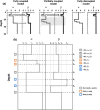
Figure 1

(a) Example of three 1‐D profiles for properties α and β: (left) fully coupled at depth, that is, the two profiles display the same number of interfaces, positioned at the same depths; (center) partially coupled at depth, that is, the two 1‐D profiles share two common interfaces at shallow depth, but the 1‐D profile for α presents three additional interfaces, at the depth level indicated by a gray‐shaded area; and (right) fully decoupled profiles, that is, the two 1‐D profiles display a different number of interfaces at not‐coincident depth positions. (b) A structure decoupling model for properties α and β. The model is composed of seven interfaces: k ₁=3, k ₂=2, and k ₃=2. In these examples, we are using “Depth” along one axis (here y axis), illustrating spatial variation. The same examples can be done using “Time” along x axis, to present temporal variations.

Figure 2

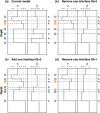
Example of models sampled along the Markov chain, following the recipe presented in this study. For sake of simplicity, model (b) is a perturbation of model (a), model (c) is a perturbation of model (b), and model (d) is a perturbation of model (c). This represents the situation where all candidate models are always accepted (i.e., prior sampling). (a) The “current” model (the same model presented in Figure 1b). Here the model is composed of seven interfaces. (b) First candidate model obtained removing one interface of “quality 3” (i.e., move 19 in our recipe: an interface with associated a value of β only). In this case, the β profile is updated, while α profile remains unchanged. (b) Next candidate obtained adding one interface of “quality 2” to the model presented in (b), move 16 in our recipe. Conversely to (b), here the α profile is updated, while β profile is left unmodified. (d) Finally, a candidate model obtained removing an interface of “quality 1”, move 15 in our recipe. Here both profiles are updated. Examples (b) and (c) illustrate some of the possible perturbations to a current model obtained using our recipe, where the two profiles are not updated simultaneously. More flexibility is given by moves 8–13 in our recipe, where profiles are perturbed with limited modification to the interface depths.

Figure 3

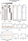
Synthetic data for the first test case: shear‐wave splitting parameters. To better illustrate how the algorithm works, we tested it using three different synthetic models. (a) Synthetic data computed using the coupled model shown in (b) as a red‐dashed line. (c) Synthetic data computed using the partially decoupled model shown in (d) as red‐dashed line. (e) Synthetic data computed using a fully decoupled model shown in (f) as a red‐dashed line.

Figure 4

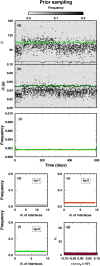
Prior sampling for the first test case. For all variables, uniform prior distributions are assumed and, thus, uniform posterior distributions are retrieved as expected. The θ (a) and δ t (b) properties. (c) The position of the interface along the x axis. Uniform priors for all classes of interfaces are retrieved. Red (class Q ₂) and gray (class Q ₁) lines are barely visible beneath the green line (class Q ₃). (d–f) The number of interfaces for each class. (g) The π parameters for the two data sets. The outlined histogram (error associated to δ t) is barely visible beneath the red histogram (error associated to θ).

Figure 5

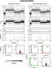
Results for the inversion of synthetic data presented in Figure 3a (fully coupled model). PPD for all the inverted parameters are shown. The panels on the left represent the results obtained using a standard joint inversion (i.e., using changepoints belonging to Q ₁ only). On the right, the panels show the results obtained with the structure decoupling algorithm. (a–d) PPD for the θ and δ t parameters. Gray‐scale colors display the PPD. Blue lines indicate mean posterior model; orange‐dashed lines indicate the true model. Black crosses show the inverted data. (e–f) Squared distance between true and mean posterior models, for θ (gray line) and δ t (gray‐dashed line). (g–h) PPD for the position of the changepoints in time. Histograms for changepoints of class Q ₁ (gray), Q ₂ (red), and Q ₃ (green). (i, k, l, and m) PPD for the number of changepoints. Histograms for changepoints of class Q ₁ (gray), Q ₂ (red), and Q ₃ (green). (j and n) PPD for the π parameters for the two data sets: δ t (outlined histograms) and θ (red histograms). PPD = posterior probability distribution.

Figure 6

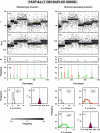
Results for the inversion of synthetic data presented in Figure 3b (partially decoupled model). See Figure 5 for symbol details.

Figure 7

Results for the inversion of synthetic data presented in Figure 3c (fully decoupled model). See Figure 5 for symbol details.

Figure 8

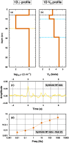
Synthetic models and data for the second test case: MT and RF data. (a and b) The ρ and V _S profiles. ρ profiles is composed of two interfaces: one interface in class Q ₁ and one interface in class Q ₂. The V _S profile is composed of three interfaces. One interface in class Q ₁ (the interface shared with the ρ profile) and two interfaces in class Q ₃. (c) Synthetic RF data generated using the V _S model in (b). (d) Synthetic MT data generated using the ρ model in (a). In both cases, we added noise to the synthetics as described in the text. MT = magnetotelluric; RF = receiver function.

Figure 9

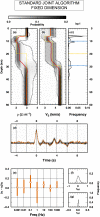
Results for the inversion of synthetic data presented in Figure 8 using a fixed‐dimensional algorithm. Here the number of interfaces is fixed to 3. Results are presented in term of PPDs. (a and b) PPD for the ρ (a) and V _S (b) properties. Gray colors represent probabilities. Yellow‐dashed lines indicate the “true” models. Red lines show the posterior mean models. Black‐dotted lines display 90% confidence level. (c) PPD for the depth of the four interfaces. Horizontal‐dashed lines indicate the position of the interfaces in the true model: gray = interfaces in class Q ₁, yellow = interfaces in class Q ₂, and blue = interfaces in class Q ₃. (d) Fit between RF data and prediction computed along the Monte Carlo sampling. A red line indicates the “observed” RF from Figure 8c. Gray colors indicate PPD if the synthetics. (e) Fit between observed and synthetic magnetotelluric data, expressed in terms of relative deviations form the observed value. The open diamonds represent the mean posterior relative deviation for each frequency; the red vertical bars indicate the 2σ interval for the posterior relative deviation. (f and g) PPD for the scale value of the errors for magnetotelluric data (f) and RF data (g). RF = receiver function; PPD = posterior probability distribution.

Figure 10

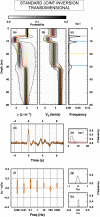
Results for the inversion of synthetic data presented in Figure 8 using trans‐dimensional algorithm. Results are presented in term of posterior probability distributions. Details for (a) to (d) as in Figure 9. (e) Posterior probability distribution of the number of interfaces. The red line indicates the uniform prior distribution. (f) as in (e) in Figure 9. (g) and (h) as in (f) and (g) in Figure 9, respectively.

Figure 11

Results for the inversion of synthetic data presented in Figure 8 using the structure decoupling algorithm. Results are presented in term of PPDs. Details for (a) and (b) as in Figure 9. (d and e) PPD for the number of interfaces in class Q ₁ (c), class Q ₂ (d), and class Q ₃ (e). Red lines indicate the prior uniform distribution. Dashed lines represent the position of the interfaces in the “true” model. (f) as in (d) in Figure 9. (g–i) PPD of the number of interfaces in class Q ₁ (g), class Q ₂ (h), and class Q ₃ (i). (j) as in (e) in Figure 9. (k) and (l) as in (f) and (g) in Figure 9, respectively. PPD = posterior probability distribution.

Figure 12

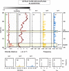
Borehole data used in the real‐world test case: reversed delay time (DTR) and electromagnetic array log (EAL). (a and b) The DTR and EAL data in the observed depth range (280–320 m). (c) Lithostratigraphy from the same borehole and depth range. Colors denote formations: coal = black, coaly shale = gray, carbonate mudstone = dark magenta; claystone = cyan, sandstone = yellow; silt = purple; dolerite = dark orange, and tuff = red. Names indicate the position of the formations cited in the main text.

Figure 13

Results for the inversion of borehole data. In (a–e), the two red boxes indicated the depth range for the formations examined in the main text. (a and b) Posterior realization of the reversed delay time (a) and electromagnetic array log (b). Gray colors indicate probability. Red lines are mean posterior models. (c–e) Posterior distribution of the interfaces at depth for Q ₁ (c), Q ₂ (d), and Q ₃ (e). Posterior distribution for the number of interfaces for Q ₁ (f), Q ₂ (g), and Q _h (h). Posterior distribution for the scaling factor π _X of the uncertainties, where X is reversed delay time (i) or electromagnetic array log (j). Scaling factor is computed as 10^π _X.

References

1. Amato, A. , Bianchi, I. , & Piana Agostinetti, N. (2014). Apulian crust: Top to bottom. Journal of Geodynamics, 82, 125–137. 10.1016/j.jog.2014.09.007 - DOI
1. Backus, G. E. (1988). Comparing hard and soft prior bounds in geophysical inverse problems. Geophysical Journal International, 94, 249–261.
1. Bayes, T. (1763). An essay towards solving a problem in the doctrine of chances. Philosophical Transactions of the Royal Society of London, 53, 370–418.
1. Bedrosian, P. A. , Maercklin, N. , Weckmann, U. , Bartov, Y. , Ryberg, T. , & Ritter, O. (2007). Lithology‐derived structure classification from the joint interpretation of magnetotelluric and seismic models. Geophysical Journal International, 170(2), 737–748. 10.1111/j.1365-246X.2007.03440.x - DOI
1. Bodin, T. , Leiva, J. , Romanowicz, B. , Maupin, V. , & Yuan, H. (2016). Imaging anisotropic layering with Bayesian inversion of multiple data types. Geophysical Journal International, 206(1), 605–629. 10.1093/gji/ggw124 - DOI
LinkOut - more resources