Protection of tissue physicochemical properties using polyfunctional crosslinkers

Abstract

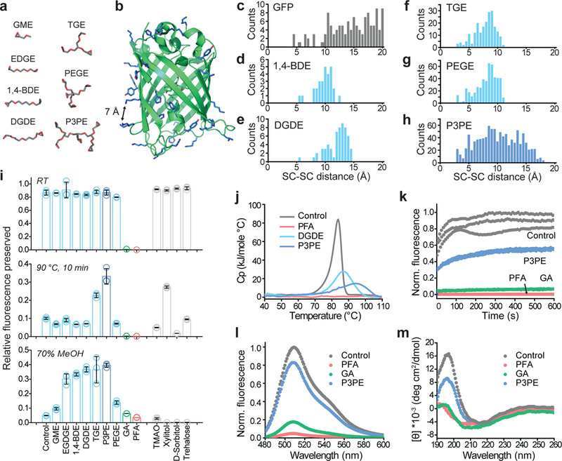
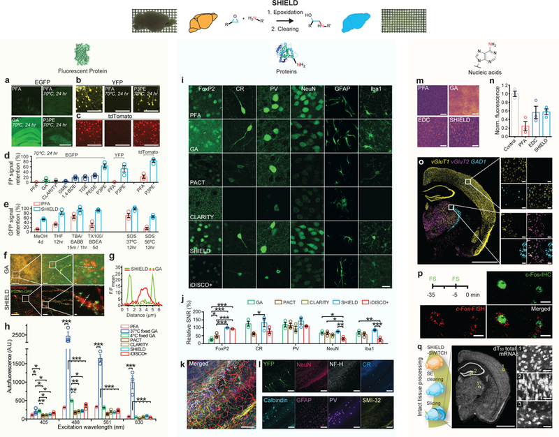
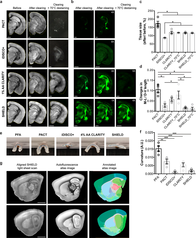
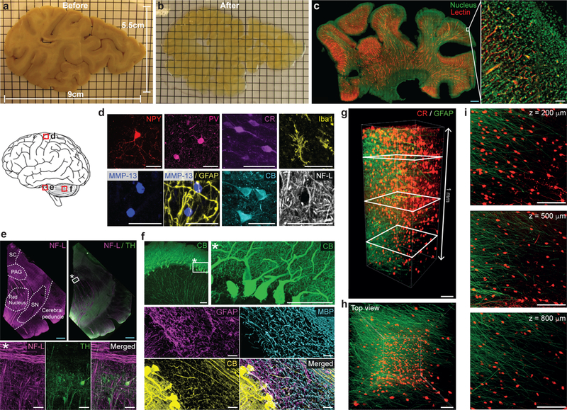
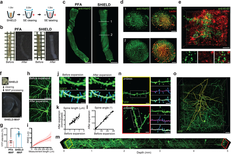
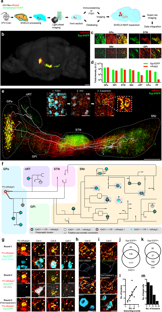
Understanding complex biological systems requires the system-wide characterization of both molecular and cellular features. Existing methods for spatial mapping of biomolecules in intact tissues suffer from information loss caused by degradation and tissue damage. We report a tissue transformation strategy named stabilization under harsh conditions via intramolecular epoxide linkages to prevent degradation (SHIELD), which uses a flexible polyepoxide to form controlled intra- and intermolecular cross-link with biomolecules. SHIELD preserves protein fluorescence and antigenicity, transcripts and tissue architecture under a wide range of harsh conditions. We applied SHIELD to interrogate system-level wiring, synaptic architecture, and molecular features of virally labeled neurons and their targets in mouse at single-cell resolution. We also demonstrated rapid three-dimensional phenotyping of core needle biopsies and human brain cells. SHIELD enables rapid, multiscale, integrated molecular phenotyping of both animal and clinical tissues.

Figure 1.. Protection of green fluorescent protein (GFP) activity with polyepoxide crosslinkers.

(a) Representative lowest-energy conformers of epoxide molecules, drawn at the same scale as b. (b) GFP structure, with epoxide-reactive residues labeled in blue. The black arrow indicates a 7-Å distance between side-chains. (c) Frequency count calculated for solvent-exposed GFP side-chains (SC) as a function of their pairwise distances. (d-h) Frequency count of the average distance between epoxide groups, determined from the lowest-energy epoxide conformers. (i) Degree of GFP fluorescence preserved after reaction with the crosslinker (top) followed by exposure to 90°C for 10 min (middle) or 70% methanol incubation for 1 hr (bottom). N=3 independent experiments. Mean +/− standard error mean was used for plotting this graph. (j) Differential scanning calorimetry plot of heat capacity as a function of the temperature of crosslinked GFP. (k) Plot of the fluorescence of crosslinked GFP recovered over time after renaturation from acid-denaturation. (l) Fluorescence spectra of crosslinked GFP. (m) Circular dichroism spectra of crosslinked GFP. GME, glycidyl methyl ether; EGDGE, ethylene glycol diglycidyl ether; 1,4-BDE, 1,4-butanediol diglycidyl ether; DGDE, dipropylene glycol diglycidyl ether; TGE, glycerol triglycidyl ether; PEGE, pentaerythritol polyglycidyl ether; P3PE, polyglycerol 3-polyglycidyl ether. PFA, paraformaldehyde; GA, glutaraldehyde. TMAO, trimethylamine N-oxide.

Figure 2.. SHIELD preserves FP signals, proteins, transcripts, and their probe-binding affinities.

(a-c) Representative FP signals of brain slices subjected to thermal treatment after processed with fixatives (PFA, GA, or P3PE). Brain slices expressing EGFP (Thy1::EGFP M-line), YFP (Thy1::YFP H-line), or tdTomato (PV-Cre / loxP-tdTomato) were used. Scale bar = 1 mm (a), 100 μm (b,c) (d) FP signal retention after the same heat treatment in brain sections preserved with difference fixatives and CLARITY. N=3 tissues. (e) GFP signal retention from M-line slices after exposure to organic solvents and detergents. MeOH, methanol; THF, tetrahydrofuran; TBA, tert-butyl alcohol; BABB, one part benzyl alcohol and two parts benzyl benzoate; TX100, Triton-X100; BDEA, butyldiethanolamine. N=3 tissues. (f) Fluorescence images of neurons virally labeled with RV-hSyn-mOrange-p2A-PSD95-GFP in GA and SHIELD tissue. Scale bars = 100, 10, and 1 μm (left to right). (g) Fluorescence intensity profiles of PSD95-GFP (green) and mOrange (red) signals along the dotted lines in f. (h) Tissue autofluorescence from various excitation wavelengths. N=3 tissues. (i) Representative images comparing the immunofluorescence of key cell-type antibodies in tissues prepared by various tissue processing methods. Scale bar = 20 μm. FoxP2, forkhead box protein P2; CR, calretinin; PV, parvalbumin; NeuN, neuronal nuclei; GFAP, glial fibrillary acidic protein; Iba1, ionized calcium-binding adapter molecule 1. The same imaging and display settings were used for each antibody. (j) Signal to noise ratios (SNR) of immunofluorescence in i normalized to the SNR of PFA control. N=3 tissues. (k, l) SHIELD preserves endogenous YFP fluorescence during multiple rounds of immunostaining and destaining. (k) Overlay of multi-round immunostained images. Scale bar = 100 μm. (l) Images from individual rounds. Scale bar = 100 μm. (m) Representative heatmaps of fluorescence in situ hybridization (FISH) of total mRNAs by (dT)₅₀-Cy3 in cleared PFA, EDC-CLARITY, GA, and SHIELD tissues. Scale bar = 100 μm. (n) Fluorescence intensities of dT₅₀-Cy3 FISH normalized to the signal of uncleared PFA tissues (Control), N=3 tissues. (o) FISH HCR against three mRNAs in SHIELD tissue. Scale bar = 1 mm (left) or 50 μm (right panels). (p) Dual labeling of c-Fos protein and mRNA in SHIELD tissue from a mouse foot shocked (FS) twice at 35 and 5 minutes before sacrifice. Scale bar = 10 μm. (q) Uniform preservation of transcripts in a SHIELD-processed brain hemisphere cleared with stochastic electrotransport (SE). See Supplementary video 1. Scale bar = 2 mm (left) or 100 μm (right panels). Mean +/− standard error mean was used to plot all the bar graphs. One-way ANOVA, Turkey’s multiple comparison test, *P<0.05, **P<0.01, ***P<0.001.

Figure 3.. SHIELD protects tissue architecture against physical and chemical stressors.

(a-b) Autofluorescence (a) and YFP (b) images of 1 mm-thick brain blocks before and after clearing, and after additional 70°C destaining step (2 hr in 300 mM SDS). The yellow dotted lines mark the original contour of the blocks before clearing. Numbers in YFP images indicate intensity gain by adjusting the display range of the images. Scale bars = 1 mm. (c) Tissue size change after delipidation and optical clearing. CLARITY_70°C indicates 1% AA CLARITY tissue destained at 70°C for 2 hr after 37°C delipidation. N=4 tissues. (d) Tissue deformation quantified by changes in the ratio of medio-lateral (M-V) and dorso-ventral (D-V) length of tissue block. N=4 tissues. (e) Photos of cleared 1 mm-thick mouse brain sagittal blocks on a rod. Interpolated centerlines of the tissues were marked with dots. (f) Quantification of tissue curvature. N=3 tissues. (g) Fully automated registration of autofluorescence images from a SHIELD mouse brain sample to autofluorescence images of Allen brain atlas (© 2015 Allen Institute for Brain Science. Allen Brain Atlas API. Available from: brain-map.org/api/index.html). Scale bar = 2 mm. Mean +/− standard error mean was used for all the bar graphs. One-way ANOVA, Turkey’s multiple comparison test, *P<0.05, **P<0.01, ***P<0.001.

Figure 4.. SHIELD enables 3D imaging of various structures and cell-types and their morphological details in human brain tissue.

(a-b) 2 mm-thick slab of human brain coronal hemisphere (9 cm × 5.5 cm × 2 mm) before (a) and after (b) SHIELD processing. Grid = 5 mm. (c) A SHIELD-processed slab (22 mm × 38 mm × 1.3 mm) was stained with lectin and nuclear dye, and the 800μm-thick volume from the top surface was imaged with a custom-built temporally focused line-scanning two-photon microscope. Scale bars = 2 mm (blue) or 100 μm (white). See Supplementary video 3. (d-f) Immunostained cortex (d), midbrain (e), and cerebellum (f) from 100-μm-thick SHIELD-processed human brain tissues showing various cell-types and structures. In e, neurofilament-L (NF-L) staining assists delineation of midbrain areas. MMP-13, matrix metallopeptidase 13; SC, superior colliculus; PAG, periaqueductal gray; SN, substantia nigra; MBP, myelin basic protein; TH, tyrosine hydroxylase; Scale bar = 2 mm (blue) or 50 μm (white). (g-i) GFAP (green) and CR (red) immunolabeling of a SHIELD-processed 1 mm-thick human cortex coronal block. See Supplementary video 4. (g) 3D reconstruction. Scale bar = 100 μm. (h) Top view of the 3D reconstruction. Scale bar = 100 μm. (i) Maximum intensity projection images at various z-positions (200, 500, and 800 μm) marked by white rectangles in g. For maximum intensity projection, 100 μm-thick z-stacks were used at each z-position. Scale bar = 100 μm.

Figure 5.. SHIELD enables new tissue phenotyping approaches.

(a-e) Ultrafast 3D molecular phenotyping of intact needle biopsy. (a) Pipeline. (b) Morphological preservation of a fresh brain biopsy by SHIELD after clearing. Grid = 1 mm; Scale bar = 1 mm. (c) Complete immunolabeling and visualization of an intact biopsy sample with Histone H3 antibody (anti-HisH3). Scale bar = 1 mm. See Supplementary video 5. (d) Cross-sectional images of c. Note that antibody and lectin signal is uniform throughout the entire volume. Scale bar = 200 μm. (e) A mouse kidney biopsy harboring breast cancer metastasis was rapidly processed and stained for a cancer cell marker (anti-Ki-67 antibody). Scale bar = 200 μm (top), 20 μm (bottom, zoom-in images). See Supplementary video 6. (f-o) Superresolution imaging of endogenous FP signal in large tissue volumes by SHIELD-MAP. (f) SHIELD-MAP pipeline and processed tissue images. (g) Fluorescence retention after PFA-MAP and SHIELD-MAP. N=4 tissues. Mean +/− standard error mean was used for plotting this graph. (h) Images showing a GFP-expressing neuron before (top) and after (bottom) SHIELD-MAP processing and expansion. Scale bar = 50 μm. (i) Root-mean-squared measurement error (RMSE) of the images before and after SHIELD-MAP processing and expansion (red line, mean; filled area, s.d.; N = 4 tissues). (j) Images showing segmented EGFP-expressing dendritic spines (blue) before and after SHIELD-MAP expansion. Scale bar = 2 μm. (k-l) SHIELD-MAP preserves morphological features of the spine, such as length (k) and angle (l) Spine length after expansion is normalized by the tissue expansion ratio. Linear regression, R² = 0.7764 (k) and R² = 0.9879 (l) N=49 and 62 spines for k and l, respectively. (m-n) Volumetric imaging of 5 mm-thick expanded SHIELD-MAP tissue. See Supplementary video 7. (n) Images showing segmented dendrites (magenta) and spines (blue) from the tissue surface (top) and at a depth of 5 mm (bottom; 1.67 mm pre-expansion). Scale bars = 10 μm. (o) Reconstructed dendrites (yellow) of a cortical Thy1-YFP⁺ neuron. Scale bar = 200 μm. See Supplementary video 8. Unpaired T-test, *P<0.05.

Figure 6.. SHIELD enables integrated circuit reconstruction at single cell resolution.

(a) Pipeline. (b) 3D rendering of the intact mouse hemisphere showing brain-wide projection patterns of labeled GPe-PV⁺ neurons. See Supplementary video 9. (c) Representative images of labeled neurons and their pre-synaptic terminals in GPe, STN, SNr, and GPi. (d) Total pixel intensity of mRuby2 and EGFP in seven brain regions to which the labeled GPe-PV⁺ neurons project. (e) 3D rendering of labeled GPe-PV⁺ neuronal circuitry with the overlaid axon trace of a single labeled neuron. The inset shows example images from multiround staining and multiscale imaging. Scale bar = 1 mm (50 μm for insets). (f) Reconstructed axon arborization of the neuron and its downstream targets. Each circle represents a neuron. The number of putative axosomatic boutons is marked inside each circle. (g) Images of the circuit components from multiround imaging. The arrow indicates the target cell body. Scale bars = 20 μm. (h) Reconstructed putative axosomatic connectivity. Ramified axons (gray) and EGFP⁺ presynaptic boutons (blue) are segmented. Scale bars = 20 μm. (i) Convergence of two axon collaterals branched remotely from the target cell body. See Supplementary video 11 for a 3D reconstruction of this connectivity. (j-k) Venn diagram showing three different neuronal populations in the SNr. (j) GAD1⁺ / Syp-EGFP⁻, GAD1⁺ / Syp-EGFP⁺, and GAD1⁻ / Syp-EGFP⁺. (k) CR⁺ / Syp-EGFP⁻, CR⁺ / Syp-EGFP⁺, and CR⁻ / Syp-EGFP⁺. Unbiased sampling was used. (l) A relationship between the number of axosomatic boutons and the axonal branching events of the reconstructed PV-mRuby2⁺ neuron near the target neuronal soma. Linear regression, R = 0.55, F-test = 17.40, P = 0.0009. N=11 connections. (m) The distribution of the number of putative axosomatic boutons. Mean +/− standard error mean was used for all the bar graphs.

References

1. Masland RH Neuronal cell types. Current Biology 14, R497–R500 (2004). - PubMed
1. Kepecs A & Fishell G Interneuron cell types are fit to function. Nature 505, 318–326 (2014). - PMC - PubMed
1. Alivisatos AP et al. The brain activity map. Science 339, 1284–1285 (2013). - PMC - PubMed
1. DeFelipe J From the connectome to the synaptome: an epic love story. Science 330, 1198–1201 (2010). - PubMed
1. Zingg B et al. Neural networks of the mouse neocortex. Cell 156, 1096–1111 (2014). - PMC - PubMed