Fast animal pose estimation using deep neural networks

Abstract

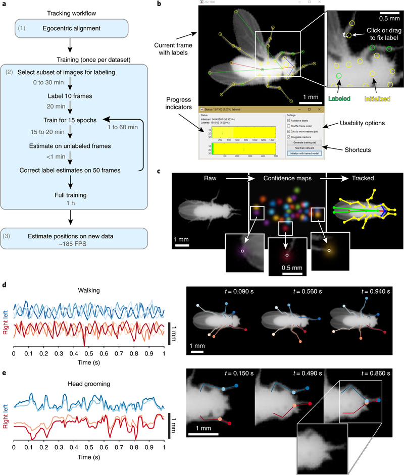
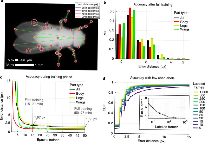
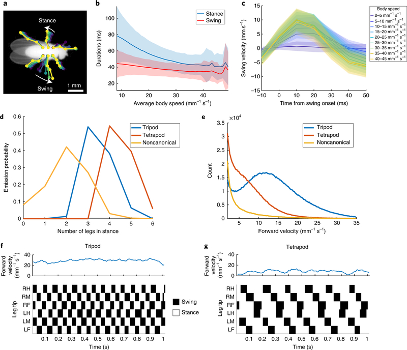
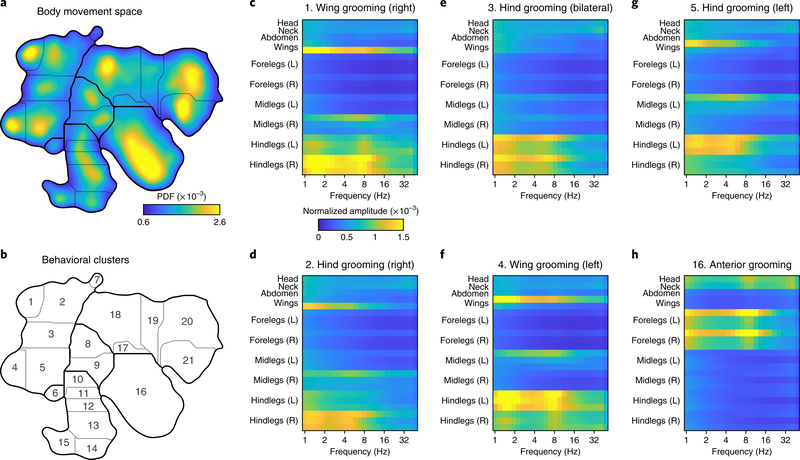
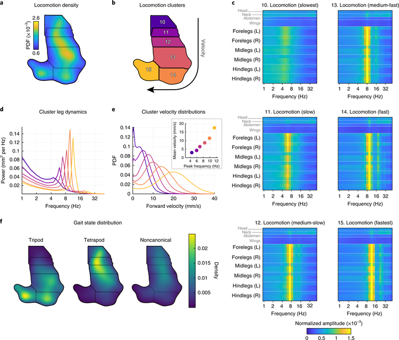
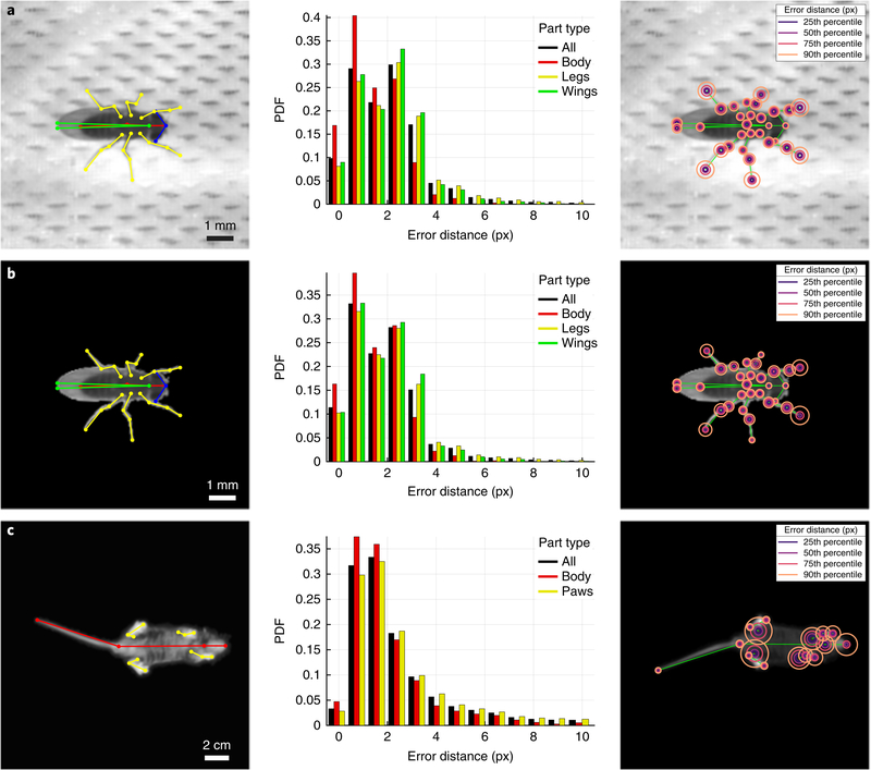
The need for automated and efficient systems for tracking full animal pose has increased with the complexity of behavioral data and analyses. Here we introduce LEAP (LEAP estimates animal pose), a deep-learning-based method for predicting the positions of animal body parts. This framework consists of a graphical interface for labeling of body parts and training the network. LEAP offers fast prediction on new data, and training with as few as 100 frames results in 95% of peak performance. We validated LEAP using videos of freely behaving fruit flies and tracked 32 distinct points to describe the pose of the head, body, wings and legs, with an error rate of <3% of body length. We recapitulated reported findings on insect gait dynamics and demonstrated LEAP's applicability for unsupervised behavioral classification. Finally, we extended the method to more challenging imaging situations and videos of freely moving mice.

Fig. 1 |. Body-part tracking via LEAP, a deep learning framework for animal pose estimation.

a, Overview of the tracking workflow. b, GUI for labeling images. Interactive markers denote the default or best estimate for each body part (top left). Users click or drag the markers to the correct location (top right). Colors indicate labeling progress and denote whether the marker is at the default or estimated position (yellow) or has been updated by the user (green). Progress indicators mark which frames and body parts have been labeled thus far, while shortcut buttons enable the user to export the labels to use a trained network to initialize unlabeled body parts with automated estimates. c, Data flow through the LEAP pipeline. For each raw input image (left), the network outputs a stack of confidence maps (middle). Colors in the confidence maps represent the probability distribution for each individual body part. Insets overlay individual confidence maps on the image to reveal how confidence density is centered on each body part, with the peak indicated by a circle. The peak value in each confidence map predicts the coordinate for each body part (right). d, Quantification of walking behavior using leg tip trajectories. The distance of each of the six leg tips from its own mean position during a walking bout as a function of time (left). Poses at the indicated time points (right). Blue and red traces correspond to left and right leg tips, respectively. e, Quantitative description of head grooming behavior described by leg tip trajectories. Position estimates are not confounded by occlusions when the legs pass under the head (right, inset).

Fig. 2 |. LEAP is accurate and requires little training or labeled data.

a, Part-wise accuracy distribution after full training. Circles are plotted on a reference image to indicate the fraction of held-out testing data (168 images from seven held-out flies) for which estimated positions of the particular body part are closer to the ground truth than the radii. Scale bars indicate image and physical size; 35 px is equivalent to 1 mm at this resolution. b, Accuracy summary on held-out test set after full training. PDF, probability density function. c, Accuracy as a function of training time. In the ‘fast training’ regime, n = 1,215 labeled frames were used for training. Lines and shaded area (smaller than line width) indicate the mean and s.e.m. for all held-out test images pooled over five runs. Run time estimates based on high-end consumer or enterprise GPUs. d, Accuracy as a function of the number of training examples. Distributions indicate estimation errors in a held-out test set (n = 168 frames) with varying numbers of labeled images used for training, pooled over five ‘fast training’ runs. CDF, cumulative distribution function. Inset: median overall r.m.s. error over these five replicates at each sample size.

Fig. 3 |. LEAP recapitulates known gait patterning in flies.

a, Schematic of swing and stance encoding. Stance is defined by a negative horizontal velocity in egocentric coordinates. b, Duration of swing and stance as a function of average body speed. These data comprise approximately 7.2 h in which the fly was moving forward (2.6 million frames). Shaded regions indicate 1 s.d. c, Swing velocity as a function of time from swing onset, and binned by body speed (n = 1,868,732 swing bouts across all legs). Shaded regions indicate 1 s.d. d, Emission probabilities of numbers of legs in stance for each hidden state in the HMM (Methods). Hidden state emissions resemble tripod, tetrapod and noncanonical gaits. e, Distributions of velocities for each hidden state. f,g, Examples of tripod (f) and tetrapod (g) gaits identified by the HMM. RH, right hind leg tip; RM, right mid; RF, right fore; LH, left hind; LM, left mid; LF, left fore.

Fig. 4 |. Unsupervised embedding of body position dynamics.

a, Density of freely moving fly body-part trajectories, after projection of their spectrograms into two dimensions via unsupervised nonlinear manifold embedding. The distribution shown was generated from 21.1 million frames. Regions in the space with higher density correspond to stereotyped movement patterns, whereas low-density regions form natural divisions between distinct dynamics. A watershed algorithm was used to separate the peaks in the probability distribution (Methods). b, Cluster boundaries from a with cluster numbers indicated. c–h, Average spectrograms for the indicated body parts from time points that fall within the dominant grooming clusters; cluster numbers are indicated in b. Qualitative labels for each cluster based on visual inspection are provided for convenience. Color map corresponds to normalized power for each body part.

Fig. 5 |. Locomotor clusters in behavior space separate distinct gait modes.

a,b, Density (a) and cluster (b) labels of locomotion clusters (from the same behavioral space shown in Fig. 4a). c, Average spectrograms (similar to Fig. 4c–h) quantifying the dynamics in each cluster. d, Average power spectra calculated from the leg joint positions for each cluster in c. Colors correspond to the cluster numbers in b. e, The distribution of forward locomotion velocity as a function of cluster number. Colors correspond to cluster numbers in b. Inset, forward locomotion velocity as a function of peak leg frequency. f, Gait modes identified by HMM from swing/stance state correspond to distinct clusters.

Fig. 6 |. LEAP generalizes to images with complex backgrounds or of other animals.

a, LEAP estimates on a separate dataset of 42 freely moving male flies, each imaged against a heterogeneous background of mesh and microphones, with side illumination (~4.2 million frames, ~11.7 h). 32 body parts (Supplementary Fig. 4) were tracked, and 1,530 labeled frames were used for training. Error rates for position estimates were calculated on a held-out test set of 400 frames (center) and were comparable to those achieved for images with higher signal to noise (compare with Fig. 2b). Part-wise error distances (right). b, LEAP estimates on masked images from the dataset described in a. Background was subtracted using standard image processing algorithms (Methods) to reduce the effect of background artifacts. c, LEAP estimates on a dataset of freely moving mice imaged from below (~3 million frames, ~4.8 h). Three points are tracked per leg, in addition to the tip of the snout, neck, and base and tip of the tail (left)—1,000 labeled frames were used for training. Accuracy rates on a held-out test set (of 242 frames) (center).

References

1. Anderson DJ & Perona P Toward a science of computational ethology. Neuron 84, 18–31 (2014). - PubMed
1. Szigeti B, Stone T & Webb B Inconsistencies in C. elegans behavioural annotation. Preprint at bioRxiv https://www.biorxiv.org/content/early/2016/07/29/066787 (2016).
1. Branson K, Robie AA, Bender J, Perona P & Dickinson MH High-throughput ethomics in large groups of Drosophila. Nat. Methods 6, 451–457 (2009). - PMC - PubMed
1. Swierczek NA, Giles AC, Rankin CH & Kerr RA High-throughput behavioral analysis in C. elegans. Nat. Methods 8, 592–598 (2011). - PMC - PubMed
1. Deng Y, Coen P, Sun M & Shaevitz JW Efficient multiple object tracking using mutually repulsive active membranes. PLoS ONE 8, e65769 (2013). - PMC - PubMed
Publication types
LinkOut - more resources