Circuit Models of Low-Dimensional Shared Variability in Cortical Networks

Abstract

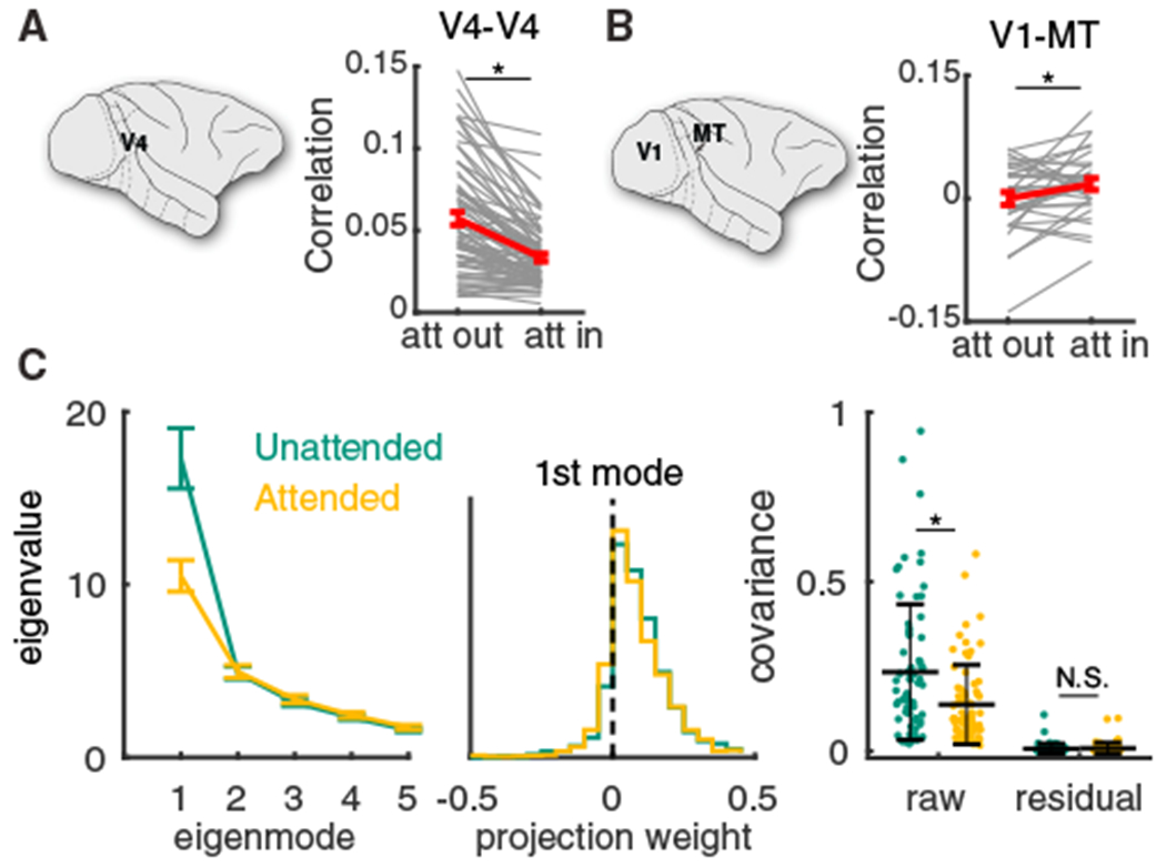
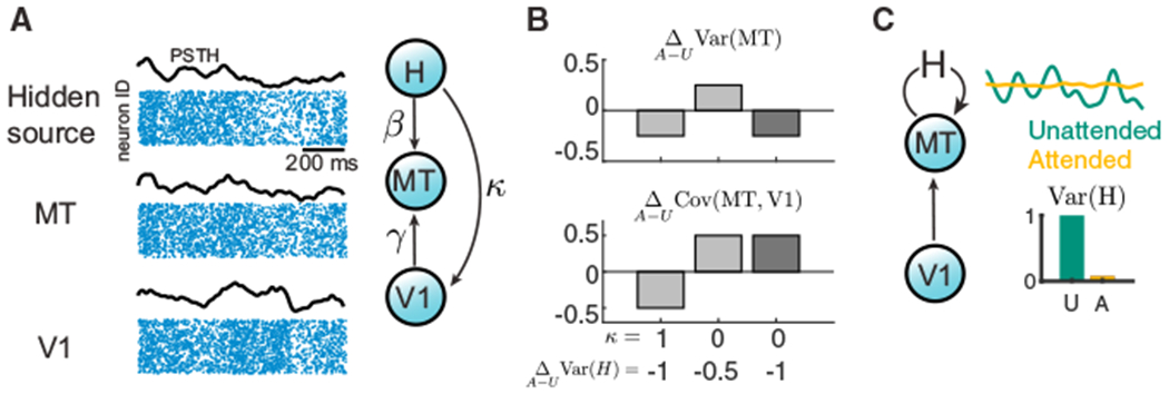
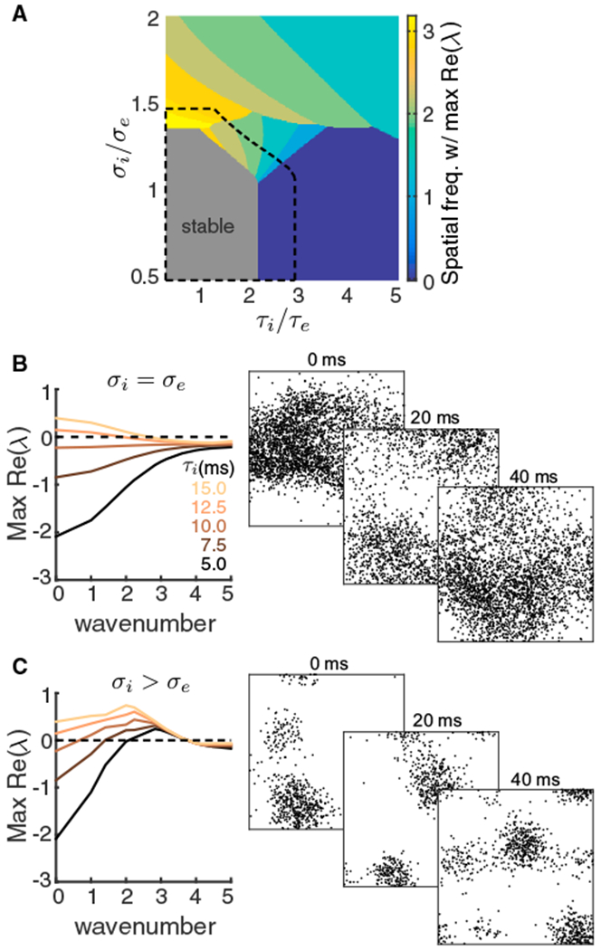
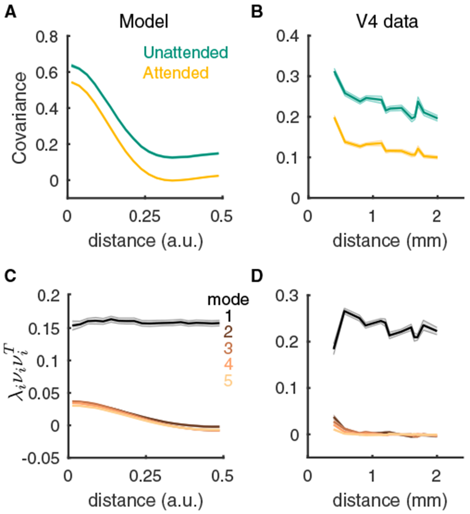
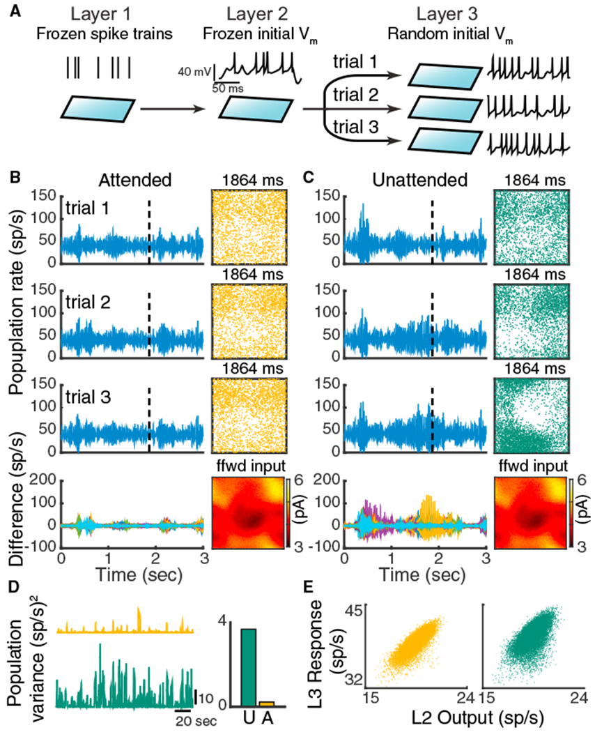
Trial-to-trial variability is a reflection of the circuitry and cellular physiology that make up a neuronal network. A pervasive yet puzzling feature of cortical circuits is that despite their complex wiring, population-wide shared spiking variability is low dimensional. Previous model cortical networks cannot explain this global variability, and rather assume it is from external sources. We show that if the spatial and temporal scales of inhibitory coupling match known physiology, networks of model spiking neurons internally generate low-dimensional shared variability that captures population activity recorded in vivo. Shifting spatial attention into the receptive field of visual neurons has been shown to differentially modulate shared variability within and between brain areas. A top-down modulation of inhibitory neurons in our network provides a parsimonious mechanism for this attentional modulation. Our work provides a critical link between observed cortical circuit structure and realistic shared neuronal variability and its modulation.

Keywords: attention; cortical model; excitatory/inhibitory balance; low dimensional; neuronal variability; noise correlations.

Figure 1.. Attentional Modulation of Population Variability within and between Cortical Areas

(A) Mean spike count correlation r_SC per session obtained from multi-electrode array recording from V4 was smaller when attention was directed into the receptive fields of recorded neurons (n = 74 sessions, two-sided Wilcoxon rank-sum test between attentional states, p = 3.3 × 10⁻⁶; reproduced from Cohen and Maunsell, 2009). Gray lines are individual session comparisons and the red line is the mean comparison across all sessions (error bars represent the SEM). (B) Same as (A) for the mean spike count correlation r_SC between V1 units and MT units per session (n = 32 sessions, paired-sample t test, p = 0.0222; data reproduced from Ruff and Cohen, 2016a). (C) Left: the first five largest eigenvalues of the shared component of the spike count covariance matrix from the V4 data (Cohen and Maunsell, 2009). Green, unattended; orange, attended; data from n = 72 sessions with 43 ± 15 neurons. Error bars are SEM. Middle: the vector elements for the first (dominant) eigenmode. Right: the mean covariance from each session in attended and unattended states before (raw) and after (residual) subtracting the first eigenmode (mean ± SD in black). Two-sided Wilcoxon rank-sum test (attended versus unattended), mean covariance, p = 1.3 × 10⁻³; residual, p = 0.75.

Figure 2.. Model Constraints for Shared Variability within and between Areas

(A) Left: hidden variable model for connected cortical areas, V1 and MT, where the response variability of MT comes from both its upstream area V1 and a hidden source H. Due to the low-dimensional structure of shared variability in population activity (Figure 1C), we use the mean population rate (black curves) to represent the population spiking activity from each area (blue dot rasters). Right: the hidden source H projects to MT and V1 with strengths β and κ, respectively. The feedforward projection strength from V1 to MT is γ. (B) Examples of attentional changes in the variance of MT, $\underset{A-U}{\Delta }\mathrm{Var}\left(\mathrm{MT}\right)$, and the covariance between MT and V1, $\underset{A-U}{\Delta }\mathrm{Cov}\left(\mathrm{MT},\text{V}1\right)$. We consider combinations of shared H (κ = 1) versus private H (κ = 0) and a moderate reduction in hidden variability $\left(\underset{A-U}{\Delta }\mathrm{Var}\left(H\right)=-0.5\right)$ versus a large reduction $\left(\underset{A-U}{\Delta }\mathrm{Var}\left(H\right)=-1\right)$. Attention-mediated simultaneous decreases in Var(MT) and increase in Cov(MT, V1) occur for private variability with a large reduction in hidden variability (dark gray). The other combinations cause a shift in the same direction for within and between area variability (light gray). Other model parameters are γ^U = 0.5, γ^A = 1, Var^U(H) = 1, β = 1, and Var(V1) = 1, independent of attentional state. U, unattended; A, attended. For general analysis, see Methods S1. (C) The differential modulation of shared variability within and between areas (Figures 1A and 1B) suggests the hidden variable H is internally generated within area MT and that attention should quench the variance of H substantially.

Figure 3.. The Spatial and Temporal Scales of Synaptic Coupling Determine Internally Generated Variability

(A) Networks of excitatory and inhibitory neuron models were simulated with either disordered connectivity (Ai and Aiii) or spatially ordered connectivity (Aii and Aiv), and with either fast inhibition (τ_i = 1 ms; Ai and Aii) or slow inhibition (τ_i = 8 ms; Aiii and Aiv). The integral of inhibitory postsynaptic current overtime is conserved as we change τ_i. In all models the timescale of excitation was τ_e = 5 ms. In the disordered networks, spike train rasters assume no particular neuron ordering. In the spatially ordered networks, three consecutive spike raster snapshots are shown with a dot indicating that the neuron at spatial position (x, y) fired within 1 ms of the time stamp. (B) Distributions of firing rates of excitatory neurons in the disordered (top) and spatially ordered (bottom) models, with faster inhibitory kinetics (purple) compared to slower inhibitory kinetics (green). (C) Same as (B) for the distributions of pairwise correlations among the excitatory population. (D) Mean correlation among the excitatory population as a function of the inhibitory decay time constant (τ_i). (E) Pairwise correlation as a function of distance between neuron pairs for spatially ordered models with slower inhibitory kinetics (green) compared to faster inhibitory kinetics (purple).

Figure 4.. Top-Down Depolarization of MT Inhibitory Neurons Captures the Differential Attentional Modulation of Shared Variability within and across V1 and MT

(A) Thalamus, V1, and MT are modeled in a three-layer hierarchy of spatially ordered balanced networks. Top-down attentional modulation is modeled as a depolarization of static current, μ_l, to MT inhibitory neurons. In both V1 and MT the recurrent projections are broader than feedforward projections (V1, ${\alpha }_{\text{ffwd}}^{\left(2\right)}=0.05,{\alpha }_{\mathrm{rec}}^{\left(2\right)}=0.1;\text{MT},{\alpha }_{\text{ffwd}}^{\left(3\right)}=0.1,{\alpha }_{\text{rec}}^{\left(3\right)}=0.2)$ and recurrent inhibition is slower than excitation (τ_i = 8 ms, τ_e = 5 ms). (B) Population averaged firing rate fluctuations from MT in the unattended state μ_l = 0.2, green) and the attended state μ_l = 0.35, orange). (C) Mean spike count correlation (r_SC) of excitatory neuron pairs in MT decreases with attentional modulation. (D) Mean r_SC between the excitatory neurons in MT and the excitatory neurons in V1 increases with attention. Error bars are SEM. (E) Left: the first five largest eigenvalues of the shared component of the spike count covariance matrix. Green, unattended; orange, attended; n = 80 sessions with 50 neurons each. Error bars are SEM. Middle: the vector elements for the first (dominant) eigenmode. Right: the mean covariance from each session in attended and unattended states before (raw) and after (residual) subtracting the first eigenmode (mean ± SD in black). Two-sided Wilcoxon rank-sum test (attended versus unattended), mean covariance, p = 1.3 × 10⁻²¹; residual, p = 3.5 × 10⁻⁸.

Figure 5.. Stability Analysis of a Two-Dimensional Firing Rate Model

(A) Bifurcation diagram of a firing rate model as a function of the inhibitory decay timescale τ_i and inhibitory projection width σ_i. The excitatory projection width and time constant are fixed at σ_e = 0.1 and τ_e = 5 ms respectively. Color represents the wavenumber with the largest real part of eigenvalue and the gray region is stable. Top-down modulation of inhibitory neurons modeling attention expands the stable region (black dashed). (B) Left: the real part of eigenvalues as a function of wavenumber for increasing τ_i, when σ_i = σ_e. Right: three consecutive spike raster snapshots of a spiking neuron network with σ_i = σ_e and slow inhibition (same network as in Figure 4 in the unattended state). (C) Same as (B) for σ_i larger than σ_e. Right: spike raster snapshots of a spiking neuron network with broad inhibitory projections, where the excitatory and the inhibitory projection widths of layer 3 were ${\alpha }_{\text{e}}^{\left(3\right)}=0.1$ and ${\alpha }_{\text{i}}^{\left(3\right)}=0.2$, respectively. Other parameters were the same as in (B).

Figure 6.. Distance Dependence of Pairwise and Population-wide Variability

(A) Pairwise covariance of spike counts from our spiking model as a function of the distance between the neurons. (B) Same as (A) but for the V4 data. Here the distance is between the electrodes that recorded the neuron pair. (C) The distance dependence functions of the first five covariance components computed from factor analysis of the model spiking activity in the unattended state. For mode i the product of the eigenmode loading onto a pair of neurons is plotted as a function of the distance between the neurons. To properly compare the modes, we scaled each curve by the eigenvalue λ_i for that mode. (D) Same as (C) but for the V4 data in the unattended state. Shaded regions are SEM. See Table S2 for the number of pairs at each distance value for the V4 data; for the model we used n = 80 sessions of 500 neurons each.

Figure 7.. Chaotic Population Firing Rate Dynamics Are Quenched by Attention

(A) Schematic of the numerical experiment. The spike train realizations in layer one and the initial states of the membrane potential of layer two neurons are identical across trials, while in each trial we randomized the initial states of the layer three neuron’s membrane potentials. (B) Three representative trials of the layer three excitatory population rates in the attended state (left, rows 1–3). Bottom row: difference of the population rates across 20 trials. Right (rows 1–3): snapshots of the neuron activity at time point 1,864 ms. Each dot is a spike within 2 ms window from the neuron at that location. Right bottom: the synaptic current each layer three neuron receives from layer two at time 1,864 ms. (C) Same as (B) for the network in the unattended state. (D) Trial-to-trial variance of layer three population rates as a function of time. Right: mean variance across time. (E) The layer three population rate tracks the layer two population rate better in the attended state. Both outputs and responses are smoothed with a 200 ms window.

References

1. Amit DJ, and Brunel N (1997). Model of global spontaneous activity and local structured activity during delay periods in the cerebral cortex. Cereb. Cortex 7, 237–252. - PubMed
1. Angulo MC, Rossier J, and Audinat E (1999). Postsynaptic glutamate receptors and integrative properties of fast-spiking interneurons in the rat neocortex. J. Neurophysiol 82, 1295–1302. - PubMed
1. Bondy AG, Haefner RM, and Cumming BG (2018). Feedback determines the structure of correlated variability in primary visual cortex. Nat. Neurosci 21, 598–606. - PMC - PubMed
1. Börgers C, and Kopell N (2005). Effects of noisy drive on rhythms in networks of excitatory and inhibitory neurons. Neural Comput 17, 557–608. - PubMed
1. Bosking WH, Zhang Y, Schofield B, and Fitzpatrick D (1997). Orientation selectivity and the arrangement of horizontal connections in tree shrew striate cortex. J. Neurosci 17, 2112–2127. - PMC - PubMed
Publication types
LinkOut - more resources