

Differential recordings of local field potential: A genuine tool to quantify functional connectivity
- PMID: 30586445
- PMCID: PMC6306170
- DOI: 10.1371/journal.pone.0209001
Differential recordings of local field potential: A genuine tool to quantify functional connectivity
Erratum in
-
Correction: Differential recordings of local field potential: A genuine tool to quantify functional connectivity.PLoS One. 2020 Jan 16;15(1):e0228147. doi: 10.1371/journal.pone.0228147. eCollection 2020. PLoS One. 2020. PMID: 31945135 Free PMC article.
Abstract
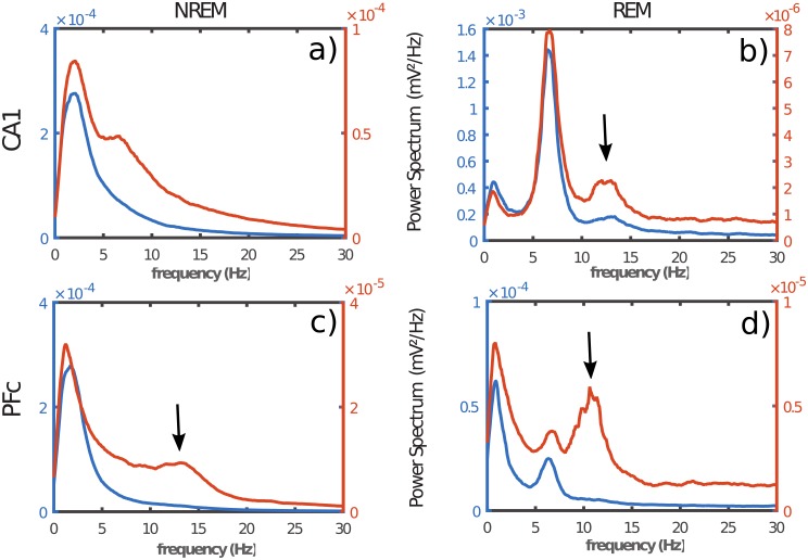
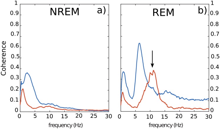
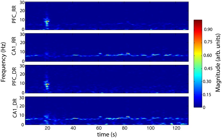
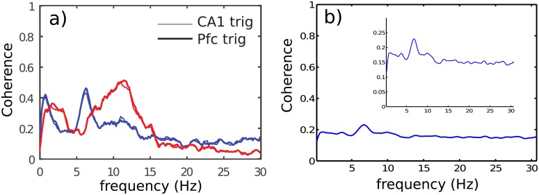
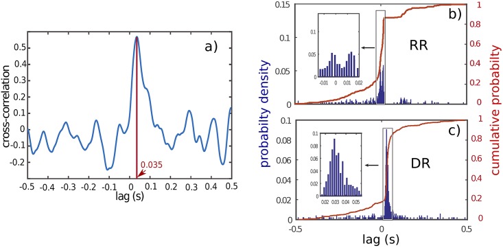
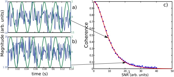
Local field potential (LFP) recording is a very useful electrophysiological method to study brain processes. However, this method is criticized for recording low frequency activity in a large area of extracellular space potentially contaminated by distal activity. Here, we theoretically and experimentally compare ground-referenced (RR) with differential recordings (DR). We analyze electrical activity in the rat cortex with these two methods. Compared with RR, DR reveals the importance of local phasic oscillatory activities and their coherence between cortical areas. Finally, we show that DR provides a more faithful assessment of functional connectivity caused by an increase in the signal to noise ratio, and of the delay in the propagation of information between two cortical structures.
Conflict of interest statement
The authors have declared that no competing interests exist.
Figures
Similar articles
-
Estimation of the effective and functional human cortical connectivity with structural equation modeling and directed transfer function applied to high-resolution EEG.Magn Reson Imaging. 2004 Dec;22(10):1457-70. doi: 10.1016/j.mri.2004.10.006. Magn Reson Imaging. 2004. PMID: 15707795
-
Electrophysiological signatures of spontaneous BOLD fluctuations in macaque prefrontal cortex.Neuroimage. 2015 Jun;113:257-67. doi: 10.1016/j.neuroimage.2015.03.062. Epub 2015 Mar 30. Neuroimage. 2015. PMID: 25837599
-
Dual Extracellular Recordings in the Mouse Hippocampus and Prefrontal Cortex.J Vis Exp. 2024 Feb 16;(204). doi: 10.3791/66003. J Vis Exp. 2024. PMID: 38436359
-
Phase correlation among rhythms present at different frequencies: spectral methods, application to microelectrode recordings from visual cortex and functional implications.Int J Psychophysiol. 1997 Jun;26(1-3):171-89. doi: 10.1016/s0167-8760(97)00763-0. Int J Psychophysiol. 1997. PMID: 9203002 Review.
-
Hippocampus as comparator: role of the two input and two output systems of the hippocampus in selection and registration of information.Hippocampus. 2001;11(5):578-98. doi: 10.1002/hipo.1073. Hippocampus. 2001. PMID: 11732710 Review.
Cited by
-
Patch-walking: Coordinated multi-pipette patch clamp for efficiently finding synaptic connections.bioRxiv [Preprint]. 2024 Aug 15:2024.03.30.587445. doi: 10.1101/2024.03.30.587445. bioRxiv. 2024. Update in: Elife. 2024 Nov 18;13:RP97399. doi: 10.7554/eLife.97399. PMID: 39185225 Free PMC article. Updated. Preprint.
-
Temporally organized representations of reward and risk in the human brain.Nat Commun. 2024 Mar 9;15(1):2162. doi: 10.1038/s41467-024-46094-1. Nat Commun. 2024. PMID: 38461343 Free PMC article.
-
Correction: Differential recordings of local field potential: A genuine tool to quantify functional connectivity.PLoS One. 2020 Jan 16;15(1):e0228147. doi: 10.1371/journal.pone.0228147. eCollection 2020. PLoS One. 2020. PMID: 31945135 Free PMC article.
-
Patch-walking, a coordinated multi-pipette patch clamp for efficiently finding synaptic connections.Elife. 2024 Nov 18;13:RP97399. doi: 10.7554/eLife.97399. Elife. 2024. PMID: 39556439 Free PMC article.
-
Mitigating Mismatch Compression in Differential Local Field Potentials.IEEE Trans Neural Syst Rehabil Eng. 2023;31:68-77. doi: 10.1109/TNSRE.2022.3217469. Epub 2023 Jan 30. IEEE Trans Neural Syst Rehabil Eng. 2023. PMID: 36288215 Free PMC article.
References
MeSH terms
LinkOut - more resources
Full Text Sources
