Sniffing Fast: Paradoxical Effects on Odor Concentration Discrimination at the Levels of Olfactory Bulb Output and Behavior

Abstract

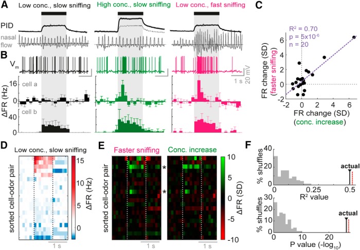
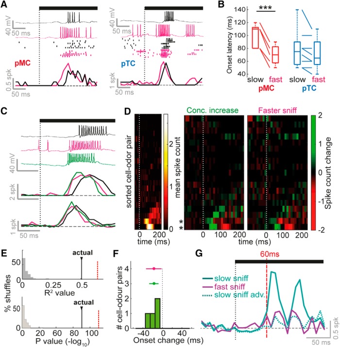
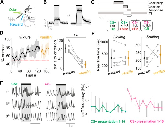
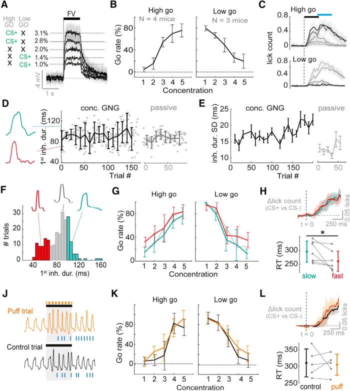
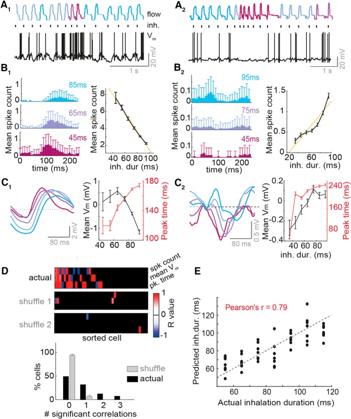
In awake mice, sniffing behavior is subject to complex contextual modulation. It has been hypothesized that variance in inhalation dynamics alters odor concentration profiles in the naris despite a constant environmental concentration. Using whole-cell recordings in the olfactory bulb of awake mice, we directly demonstrate that rapid sniffing mimics the effect of odor concentration increase at the level of both mitral and tufted cell (MTC) firing rate responses and temporal responses. Paradoxically, we find that mice are capable of discriminating fine concentration differences within short timescales despite highly variable sniffing behavior. One way that the olfactory system could differentiate between a change in sniffing and a change in concentration would be to receive information about the inhalation parameters in parallel with information about the odor. We find that the sniff-driven activity of MTCs without odor input is informative of the kind of inhalation that just occurred, allowing rapid detection of a change in inhalation. Thus, a possible reason for sniff modulation of the early olfactory system may be to directly inform downstream centers of nasal flow dynamics, so that an inference can be made about environmental concentration independent of sniff variance.

Keywords: Concentration; olfaction; olfactory bulb; oscillations; perception; sniffing.

Figure 1.

Sniff change and concentration change have very similar effects on FR responses of MTCs. A, Stimulation paradigm during whole-cell recordings. PID traces show response of photoionization detector (magnitude proportional to odor concentration), while nasal flow traces show example sniffing behavior recorded using external flow sensor for the three types of trial. See Figs. 1-1 and 1-2 for details about sniff parameters. Black bar and gray box shows where odor is applied. B, Example odor responses recorded in each stimulus condition. V_m traces show example responses for cell a, while PSTHs below show averaged FR responses in 250 ms time bins for five trials in each case. Bottom-most PSTHs are calculated for a different example, cell b. Error bars show standard deviation (SD). All are aligned to first inhalation onset after odor onset. C, Scatter plot comparing mean FR response change for concentration change and sniff frequency change (normalized by the SD of baseline FR changes in the 2 s before odor stimulus for each cell-odor pair) across first second of odor stimulus. n = 20 cell-odor pairs. D, Heatmap of average FR responses for all cell odor pairs in the low concentration, slow sniff frequency condition, ordered by mean FR response. E, Heatmap of FR response differences (difference between PSTHs) normalized by the SD of baseline FR differences in the 2 s before odor stimulus for each cell-odor pair. Concentration increase = high concentration, slow sniffing, minus low concentration, slow sniffing. Faster sniffing = low concentration, fast sniffing, minus low concentration, slow sniffing. Asterisks indicate cell a and cell b examples. F, Top: R ² values for correlations across all odor time bins as shown in E, between FR changes due to concentration change and those due to sniff frequency change. Histogram shows R ² values for shuffle controls, “actual” shows R ² value for real data. Red dotted line indicates value for correlation between FR changes due to concentration increase for two separate sets of high concentration trials. Bottom: as for above, but histogram showing p-values for the correlations (–log₁₀). See Fig. 1-3 for analysis of membrane potential responses.

Figure 2.

Faster inhalation causes temporal shifts similar to those caused by concentration increase. A, From top to bottom: example V_m traces, spike rasters, and mean spike counts for early excitatory responses for slow inhalation (black) and fast inhalation (pink), for two different cell-odor pairs. The left example is from a putative mitral cell (pMC) and the right example is from a putative tufted cell (pTC). Rasters are ordered (top to bottom) from slowest to fastest inhalation. Black bar and dotted line indicate odor onset aligned to the first inhalation onset. B, Comparison of response onset latencies for excitatory responses evoked by fast and slow sniffs for pMCs and pTCs. See also Fig. 2-1. C, Example V_m traces (above, for one cell) and mean spike counts (below, for two different cells) for early excitatory responses. Black shows response at low concentration evoked by slow inhalation, pink shows response at low concentration evoked by fast inhalation, and green shows response for high concentration evoked by slow inhalation. D, Left: heatmap to show spike counts of all 20 cell-odor pairs in response to low concentration odor stimulus and slow inhalation, for the first 250 ms of stimulation. Cell-odor pairs are sorted by the mean spike count during odor. Middle: heatmap to show difference in spike counts between high concentration and low concentration (evoked by slow inhalation). Left: heatmap to show difference in spike counts between fast inhalation and slow inhalation (low concentration stimulus). E, Top: R ² values for correlations across all odor time bins as shown in D, between spike count changes due to concentration increase and due to faster inhalation. Histogram shows values for shuffle controls (see Methods), black bars show value for actual data. Red dotted line indicates value for correlation between spike count changes due to concentration increase for two separate sets of high-concentration trials. Bottom: as for above, but histogram showing p-values for the correlations (–log₁₀). F, Histogram to show excitatory response onset latency changes due to concentration increase. Error bar in green shows mean and SD of this data, and in pink shows the distribution due to sniff changes (from dataset in panel B) for comparison. G, Euclidean distance between population spike count response vectors for high- versus low-concentration stimuli (where data for both came from slow inhalation trials; “slow sniff,” solid cyan), for high concentration and time-shifted low concentration (“slow sniff adv.,” where excitatory latency changes due to concentration change were undone via time shifting of the data; dotted cyan), and for high concentration and low concentration where low concentration data came from fast inhalation trials (“fast sniff,” solid purple).

Figure 3.

Mice rapidly learn to discriminate concentrations on fast timescales. A, Diagram of head-fixed behavior setup. B, Average PID traces for concentration go/no-go stimuli. Shaded area shows SD. See Fig. 3-1A for odor outlet flow traces. C, Concentration go/no-go task sequence. See Fig. 3-1B for training protocol. D, Left: average learning curve for eight mice. Percentage correct is calculated as a moving average over 5 CS+ and 5 CS– trials. Shaded area indicates SD. Mice are initially trained on two concentrations of an odor mixture, and subsequently tested on the same two concentrations of vanillin. Right: distribution of learning times to criterion (four successive learning curve points at or above 80% correct), for the odor mixture and vanillin. E, Left: distribution of reaction times (RTs) calculated from licking behavior for the odor mixture and vanillin. Right: as for left, but for RTs calculated from sniffing behavior (see Methods). F, Left: example sniff traces for the 1st, 3rd, and 8th presentation of the CS+ and CS– concentrations for the initial concentration discrimination learning session. Note that in this session, the CS+ concentration is first presented 10 times to ensure retention of the lick pattern learned the day before, and then the CS– is interleaved in a pseudorandom order. Right: plot to show median sniff frequency across 8 mice (regardless of concentration-reward contingency) for presentations 1–10 of the CS+ and CS– concentration in the first 2 concentration discrimination sessions. Boxes show upper and lower quartiles.

Figure 4.

Variance in inhalation has no overt impact on concentration discrimination performance. A, Diagram to show average PID traces for the five different concentrations and contingency schemes. Shaded area shows SD. To the left the contingencies are shown for “high-go” and “low-go” trained mice, with black crosses indicating CS– stimuli. B, Average go rate (percentage of trials with a go response) across mice for all five concentrations. C, Mean lick counts averaged across mice for the five different concentrations (darkest = strongest) for both “high go” and “low go” training contingencies. Black bar indicates odor stimulus, and blue bar indicates response period. D, Plot to show inhalation duration for first inhalation of the odor stimulus across trials, for the first session of one example mouse performing the five-concentration go/no-go task (“concentration GNG”), and for a passively exposed mouse (“passive”). Error bars show SD for each 10-trial block. Example representative nasal flow waveforms for single sniffs are shown to the left. E, Mean SD for the first inhalation duration (ms) during the odor stimulus, for seven mice performing five-concentration go/no-go in their first session, and for passively exposed mice (n = 23). SD is calculated for each 10-trial block of a session for each mouse. Error bars show standard error. F, Example histogram of inhalation durations of the first sniff during an odor stimulus across trials for one mouse. Data for each mouse is partitioned into fast inhalations (<30^th percentile, red), slow inhalations (>70^th percentile, cyan), and other (gray). Example representative nasal flow waveforms for a single sniff of each subset are shown. G, Go rate as a function of concentration when splitting trials according to duration of first inhalation as in F. Dotted line shows mean go rate for sniffs with inhalation between 30^th and 70^th percentile. H, Top: average difference in lick-histograms between CS+ and CS– (highest versus lowest concentration) averaged across all seven mice for slow sniff trials (cyan data) and fast sniff trials (red data) partitioned as in F. Shaded area indicates SD. Dashed line indicates odor stimulus onset aligned to the first inhalation. Bottom plot shows difference in reaction times as measured by licking for fast and slow sniff trials for all seven mice. See also Fig. 3-1D. J, Example sniff traces for one animal for a puff trial (a trial in which an air puff to the flank was used to evoke fast sniffing) and an adjacent control trial of the same concentration. Blue ticks indicate licks. K, Mean go rate as a function of concentration across mice for puff trials (orange) versus control trials (black). L, As for H, but now comparing lick distributions and reaction times between puff trials and control trials. See also Fig. 3-1E.

Figure 5.

Inhalation duration transforms mean baseline MTC activity in a large proportion of cells. A₁–C₁ refer to one example cell, while A₂–C₂ refer to a different example cell. A_1–2, Example nasal flow traces and V_m traces in absence of odor. Sniffs are color coded according to inhalation duration (blue = slow, and red = fast). Black ticks indicate inhalation onset. B_1–2, Left: average spike count histograms triggered by inhalations of different durations (denoted on each histogram). Right: mean spike count per sniff as a function of inhalation duration. Error bars = standard error (SE). C_1–2, Left: inhalation-triggered mean V_m waveforms for sniff cycles of different inhalation duration. Right: mean V_m and timing of V_m peak for membrane potential waveforms averaged across all sniffs as a function of inhalation duration. Error bars = SE. D, Top: heatmap of R values for correlations between inhalation duration and 3 different activity parameters (spike count, mean membrane potential, and timing of peak membrane potential, rows 1–3, respectively), for 45 MTCs. Cells are sorted left to right from largest number of significant correlations to lowest number. Black squares show where the correlation was insignificant (p > 0.01, linear regression). Two lowest heatmaps show the same data but for two example shuffle controls, where inhalation durations were shuffled with respect to the physiology, and the data reanalyzed. This gives an indication of false-positive rates in this analysis. Bottom: histogram to show proportion of cells with 0–3 significant correlations between the different activity parameters and inhalation duration. Gray shows proportion for shuffle controls. E, Scatter plot between inhalation duration predicted by a simple linear model using peak spike rates of 25 cells (see Methods) and the actual (true) inhalation duration for all 7 sniff cycles tested in each category. See Fig. 5-1 for the impact of cell type on responses to inhalation change, Fig. 5-2 for further analysis regarding detecting inhalation change, and Fig. 5-3 for a hypothetical relative timing code using this information to infer environmental concentration change.

References

1. Abraham NM, Spors H, Carleton A, Margrie TW, Kuner T, Schaefer AT (2004) Maintaining accuracy at the expense of speed: stimulus similarity defines odor discrimination time in mice. Neuron 44:865–876. 10.1016/S0896-6273(04)00753-6 - DOI - PubMed
1. Adrian ED (1950) The electrical activity of the mammalian olfactory bulb. Electroencephalogr Clin Neurophysiol 2:377–388. - PubMed
1. Aungst JL, Heyward PM, Puche AC, Karnup SV, Hayar A, Szabo G, Shipley MT (2003) Centre-surround inhibition among olfactory bulb glomeruli. Nature 426:623–629. 10.1038/nature02185 - DOI - PubMed
1. Banerjee A, Marbach F, Anselmi F, Koh MS, Davis MB, Garcia da Silva P, Delevich K, Oyibo HK, Gupta P, Li B, et al. (2015) An interglomerular circuit gates glomerular output and implements gain control in the mouse olfactory bulb. Neuron 87:193–207. 10.1016/j.neuron.2015.06.019 - DOI - PMC - PubMed
1. Bathellier B, Buhl DL, Accolla R, Carleton A (2008) Dynamic ensemble odor coding in the mammalian olfactory bulb: sensory information at different timescales. Neuron 57:586–598. 10.1016/j.neuron.2008.02.011 - DOI - PubMed
Publication types
LinkOut - more resources