Chronology of motor-mediated microtubule streaming

Abstract

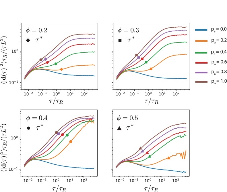
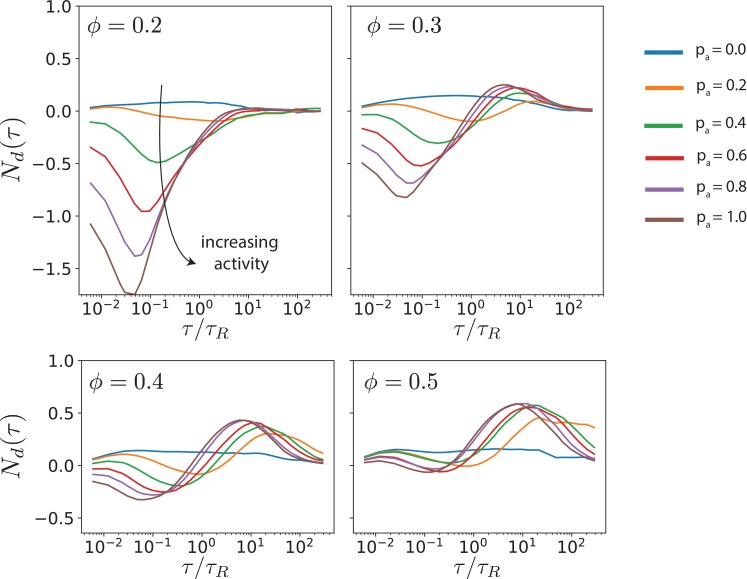
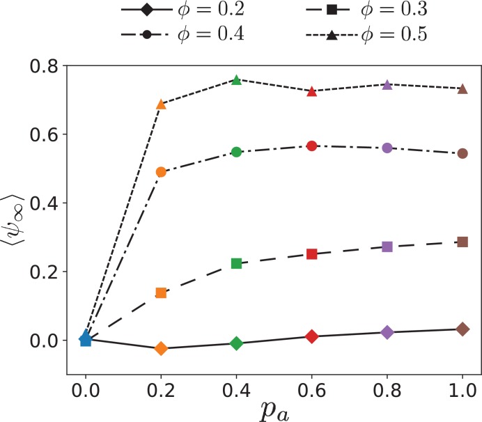
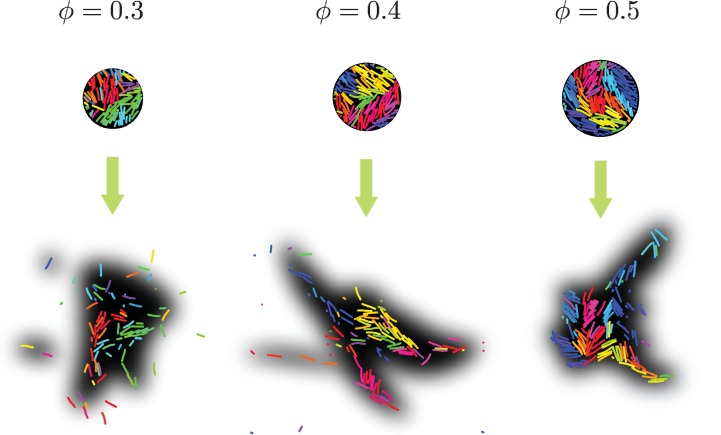
We introduce a filament-based simulation model for coarse-grained, effective motor-mediated interaction between microtubule pairs to study the time-scales that compose cytoplasmic streaming. We characterise microtubule dynamics in two-dimensional systems by chronologically arranging five distinct processes of varying duration that make up streaming, from microtubule pairs to collective dynamics. The structures found were polarity sorted due to the propulsion of antialigned microtubules. This also gave rise to the formation of large polar-aligned domains, and streaming at the domain boundaries. Correlation functions, mean squared displacements, and velocity distributions reveal a cascade of processes ultimately leading to microtubule streaming and advection, spanning multiple microtubule lengths. The characteristic times for the processes extend over three orders of magnitude from fast single-microtubule processes to slow collective processes. Our approach can be used to directly test the importance of molecular components, such as motors and crosslinking proteins between microtubules, on the collective dynamics at cellular scale.

Keywords: cell biology; computational biology; computer simulations; cytoskeletal streaming; kinesin; microtubules; molecular motors; systems biology.

Figure 1.. Schematic illustrating MT bundling and streaming.

Polar-aligned MTs are coloured blue, and antialigned MTs are coloured red. The grey/black MT is transported from its initial position (grey), in one polar-aligned bundle, to its final position (black), to another polar-aligned bundle, via a stream.

Figure 2.. Schematic explaining the conditions that satisfy the antialigned motor potential.

The vectors, ${\mathbf{𝐩}}_i$, ${\mathbf{𝐩}}_j$, and ${\mathbf{𝐦}}_{ij}$, represent the unit orientation vectors of MT $i$, MT $j$, and the motor vector that crosslinks the beads of adjacent MTs, respectively. The white circles represent the maximum extension of motors between the two MTs.

Figure 3.. Motor-driven and diffusive motion of MTs.

(a) Simulation snapshot of MTs organised by effective motors. MTs are coloured based on their orientation according to the colour legend on the right. See corresponding Video 1. (b) Trajectories of MTs within a time window of 1.2 ${\tau }_R$ separated based on the antialigned and polar-aligned categories. See corresponding Video 2. (c) Plots of the trajectory of three selected MTs coloured based on the correlation of adjacent steps in their velocity. The entire trajectory is for a time window of ${\displaystyle 300{\tau }_R}$ is the unit vector of MT displacement. The fast-streaming and slow-diffusion modes correspond with the yellow and red parts of the trajectories respectively. The scale bar corresponds to the length of five MTs. See corresponding Video 3. (d) MSD/lag time for various levels of activity $p_{\mathrm{a}}$ and MT density ${\displaystyle \varphi =0.3}$. The time scale of maximal activity, ${\tau }^{*}$, calculated from the time of maximal $v_{\parallel }$ skew is indicated by the squares on the curves. (e) Histogram of parallel velocity for various $\tau$. The curve closest corresponding to the time scale of maximal activity, ${\tau }^{*}$, is indicated with a box marker. All figures are for $\varphi =0.3$. (a), (b), (c) and (e) are for $p_{\mathrm{a}}=1.0$.

Figure 3—figure supplement 1.. Parallel velocity v∥, extrapolated to τ=0 as function of the antialigned motor probability pa for various MT surface fractions ϕ.

Figure 3—figure supplement 2.. Simulation snapshots at steady state for various antialigned motor probabilities pa and MT surface fractions ϕ.

Data for ${\displaystyle 0.0<p_{\mathrm{a}}\le 1.0}$ and ${\displaystyle 0.3<\varphi <0.5}$. The surface fractions of MTs are varied by changing the size of the periodic box, while keeping the number of MTs constant. The scale bars correspond to the length of a single MT. The colours represent the orientation of the polar MTs with respect to the system reference frame according to the colour wheel above.

Figure 3—figure supplement 3.. Translational MT mean squared displacements for various antialigned motor probilities pa and MT surface fractions ϕ.

The symbols on the plots indicate the time scale at which the parallel velocity is maximally skewed due to active forces.

Figure 3—figure supplement 4.. Parallel velocity v∥ as a function of the time window τ for various antialigned motor probabilities pa and MT surface fractions ϕ.

Figure 3—figure supplement 5.. Maximum parallel MT velocities v∥,A⁢(τ*) as function of the antialigned motor probability pa for various MT surface fractions ϕ.

Figure 3—figure supplement 6.. Histogram of v∥ for various MT surface fractions ϕ and five time windows τ.

The darkness of the curve represents the time window used to measure the parallel velocity. The darkest-coloured curve represents the parallel velocity obtained for the shortest time window, and the lightest-coloured curve is obtained from the longest time window. The box symbols mark the displacement distributions that are closest to the distribution which is most skewed.

Figure 3—figure supplement 7.. Histogram of v∥⁢(τ*) for various pa and ϕ.

The duration of the time window corresponds to the maximal skew, see Figure 6. This indicates the structure of the velocity distribution when the skew is maximal. The ordinate axis is log scaled to show the deviation of the distribution from a Gaussian, which would appear as a symmetric inverted parabola.

Figure 3—figure supplement 8.. Probability densities of the MT local polar order parameter ψi.

Data for various antialigned motor probabilities $p_{\mathrm{a}}$ and MT surface fractions $\varphi$. The arrows indicate the changes of the probability densities for increasing activity. A, M and P indicate ${\psi }_i\le -0.5$ (green), $-0.5<{\psi }_i<0.5$ (white), ${\psi }_i\ge 0.5$ (blue), respectively. $N_A$, $N_m$ and $N_P$ are the number of MTs in antialigned, perpendicular and polar-aligned environments respectively. Note that the scale of the ordinate is different for each MT surface fraction.

Figure 3—figure supplement 9.. MT parallel velocity distributions.

Data for $v_{\parallel }$ for a time window of duration ${\tau }^{*}$ and $\varphi =0.3$, decomposed based on MT environments (A, M, P) determined by their local polar order parameter, ${\psi }_i$, see Figure 8. (a) and (b) show probability density histograms of $v_{\parallel }({\tau }^{*})$ for $p_{\mathrm{a}}=0.2$ and $1.0$, respectively. (c) and (d) show frequencies of occurrence of $v_{\parallel }({\tau }^{*})$ for $p_{\mathrm{a}}=0.2$ and $1.0$, respectively. The sum of the decomposed curves in (c) and (d) gives the solid curves.

Figure 3—figure supplement 10.. MT mean squared displacements: computer simulation and experimental data.

(a) Normalized MSD curves from our simulations for several motor probabilities $p_a$. (b) Normalized MSD curves as a function of lag time for experiments eLifeMediumGrey (Sanchez et al., 2012) for selected ATP concentrations. Here $L$ is the filament length, ${\tau }_R^{\mathrm{0}}$ the single filament rotation time and $\tau$ the lag time.

Figure 4.. Displacement correlations of MTs.

(a) Spatio-temporal correlation function $C_{\mathrm{d}}(r,\tau )$ for $\varphi =0.3$ and $p_{\mathrm{a}}=1.0$, for some selected lag times. The arrow and the colours of the curves indicate increasing lag time. The lag times are picked from a logarithmic scale. (b) Neighbour correlation function $N_{\mathrm{d}}(\tau )=C_{\mathrm{d}}(\sigma ,\tau )$ for $\varphi =0.3$ and various $p_{\mathrm{a}}$ values. (c) The sliding time scale indicated by ${\tau }_{N,\min }$ is shown for various MT surface fractions and $p_{\mathrm{a}}$ values.

Figure 4—figure supplement 1.. Neighbour displacement correlation function Nd⁢(τ) for various MT surface fractions ϕ and antialigned motor probabilities pa.

The lag times at which the minimum and maximum of $N_{\mathrm{d}}(\tau )$ occur are ${\tau }_{N,\text{min}}$ and ${\tau }_{N,\text{max}}$, respectively.

Figure 5.. Local polar order of MTs.

(a) Mean local polar order $⟨{\psi }_i(\tau )⟩$ for $p_{\mathrm{a}}=0.0$ and $p_{\mathrm{a}}=1.0$ at $\varphi =0.3$, for MTs starting from antialigned (dotted line) and aligned (solid line) environments at $\tau =0$. (b) Deviation of local polar order $Q(\tau )$ for $\varphi =0.3$ for various $p_{\mathrm{a}}$ for antialigned MTs. (c) Relaxation time for the polar order parameter, ${\tau }_{Q/2}$ for various $p_{\mathrm{a}}$ and $\varphi$, estimated by the time for $Q$ to decrease to half its initial value.

Figure 5—figure supplement 1.. MTs coloured based on their local polar order parameter ψi for pa=1.0, ϕ=1.0.

The colour corresponding to $-1<{\psi }_i<1$ is given on the right. Zoomed in illustrations of MTs show examples of MTs in the three ${\psi }_i$ categories distinguished in Figure 8. The MT in question is highlighted in yellow in the zoomed in graphics. (M) ${\psi }_i\approx 0$ values can occur either when MTs are perpendicularly oriented with respect to its surrounding or when MTs have neighbours which are both polar-aligned and antialigned. (P) ${\psi }_i>0.5$ occurs when MTs have neighbours which are mostly polar-aligned. (A) ${\displaystyle {\psi }_i<-0.5}$ occurs when MTs have neighbours which are mostly antialigned.

Figure 5—figure supplement 2.. Deviation from local polar order Q⁢(τ) as function of the lag time τ for various antialigned motor probabilities pa for polar-aligned MTs.

Figure 5—figure supplement 3.. Mean local polar order parameter of MTs at long times, ⟨ψ∞⟩, for various surface fractions ϕ and antialigned motor probabilities pa.

Figure 6.. MT parallel velocity distributions.

(a) Skew of parallel velocity ($v_{\parallel }$) distribution computed as function of lag times for different $p_{\mathrm{a}}$ for $\varphi =0.3$. The probability distributions that correspond to the maximal skew are shown in Figure 3—figure supplement 6 together with distributions for few other lag times. (b) Lag time at which maximal skew is observed in the $v_{\parallel }(\tau )$ distribution (compare Figure 1). The ordinate is log-scaled to show that ${\tau }^{*}$ is exponentially decreasing with $p_{\mathrm{a}}$.

Figure 6—figure supplement 1.. Skews α3 of parallel velocity distributions (v∥) (Fig.

Figure 6) computed as a function of lag times for various antialigned motor probabilities $p_{\mathrm{a}}$ and surface fractions $\varphi$. The probability distributions that correspond to the maximal skew are shown in Figure 6 together with distributions for few other lag times. The ordinate scale is the same for comparison of the skews for different MT surface fractions.

Figure 6—figure supplement 2.. Ratios of MT populations in environments with different local polar order.

Ratios of MT populations in (a) antialigned to polar-aligned environments, and (b) perpendicular environments to total number of MTs, for various MT surface fractions $\varphi$ and antialigned motor probabilities $p_{\mathrm{a}}$.

Figure 6—figure supplement 3.. First three moments of the parallel velocity (v∥) distribution.

First three moments, (a) mean, (b) variance, (c) skew of the $v_{\parallel }$ distribution for a time window of duration ${\tau }^{*}$ for MTs in (A) antialigned, (${\psi }_i<-0.5$, blue), (P) polar-aligned (${\psi }_i>0.5$, red), and (M) mixed ($|{\psi }_i|\le 0.5$, green) environments, for different $\varphi$ and $p_{\mathrm{a}}$. The blue, red and green markers indicate moment calculated from raw data. The yellow markers are obtained from calculating moments from fits to the antialigned parallel MT velocity distribution $v_{\parallel ,A}$. (d) Example of differences in structures of $v_{\parallel }$ distributions due to increasing activity from $p_{\mathrm{a}}=0.4$ (dotted line) to $p_{\mathrm{a}}=1.0$ (solid line) for $\varphi =0.3$, for A, P and M categories of MT environment.

Figure 7.. Collective motion of MTs.

Schematic of expected evolution of photobleached regions in (a) polar-aligned and (b) antialigned regions. (c) Selectively visualised MTs in a circular region within the simulation box, and their evolution after a time of ${\tau }_{N,\max }$, for $\varphi =0.4$ and $p_{\mathrm{a}}=1.0$. The black backgrounds are predictions of FRAP results.

Figure 7—figure supplement 1.. FRAP-like predictions for various MT surface fractions ϕ.

Predictions for photobleaching experiments with $\varphi =0.3$, $0.4$, and $0.5$. MTs retain the orientation colour from when they were tagged at $t=0$. The black shadow shows our predictions for photobleaching experiments at time ${\tau }_{\mathrm{N},\max }$ after bleaching a circular patch.

Figure 8.. MT orientational correlation and active diffusion.

(a) Orientational correlation function for $\varphi =0.3$ for various antialigned motor probabilities $p_a$. (b) Inverse of rotational diffusion, ${\tau }_r$ for various antialigned motor probabilities $p_a$ and surface fractions $\varphi$ (c) Active diffusion coefficient $D_A$ for $p_{\mathrm{a}}=1$.

Figure 9.. Chronology of MT streaming. Events from antialigned MT propulsion to MT rotation (left to right) which make up the streaming process, for various antialigned motor probabilities pa and surface fractions ϕ=0.3, ϕ=0.4, and (c) ϕ=0.5 as indicated.

Author response image 1.. Mean squared displacements of filaments obtained from Langevin Dynamics (LD) and Brownian Dynamics (BD), for single filaments (left) and filaments in suspensions with packing fraction 𝜙 = 0.3 (right).

The simulation parameters are the same as in the manuscript.

References

1. Abkenar M, Marx K, Auth T, Gompper G. Collective behavior of penetrable self-propelled rods in two dimensions. Physical Review E. 2013;88:062314. doi: 10.1103/PhysRevE.88.062314. - DOI - PubMed
1. Aranson IS, Tsimring LS. Pattern formation of microtubules and motors: inelastic interaction of polar rods. Physical Review E. 2005;71:050901. doi: 10.1103/PhysRevE.71.050901. - DOI - PubMed
1. Aranson IS, Tsimring LS. Theory of self-assembly of microtubules and motors. Physical Review E. 2006;74:031915. doi: 10.1103/PhysRevE.74.031915. - DOI - PubMed
1. Axelrod D, Koppel DE, Schlessinger J, Elson E, Webb WW. Mobility measurement by analysis of fluorescence photobleaching recovery kinetics. Biophysical Journal. 1976;16:1055–1069. doi: 10.1016/S0006-3495(76)85755-4. - DOI - PMC - PubMed
1. Bates MA, Frenkel D. Phase behavior of two-dimensional hard rod fluids. The Journal of Chemical Physics. 2000;112:10034–10041. doi: 10.1063/1.481637. - DOI
Publication types