

Statistical non-parametric mapping in sensor space
- PMID: 30603166
- PMCID: PMC6208496
- DOI: 10.1007/s13534-017-0015-6
Statistical non-parametric mapping in sensor space
Abstract
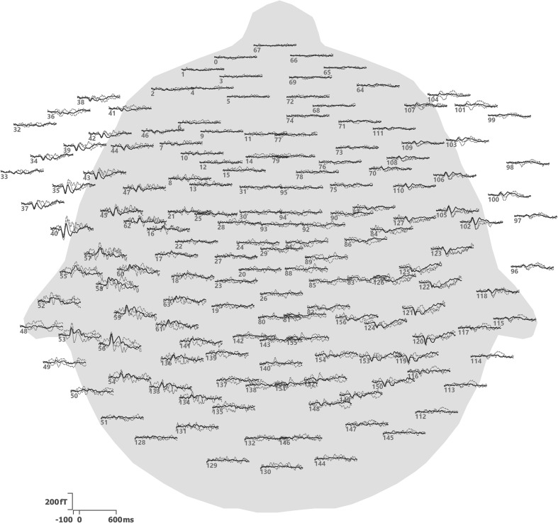
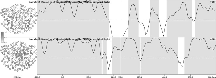
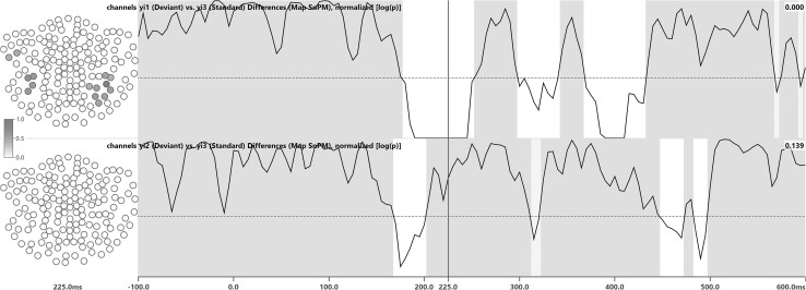
Establishing the significance of observed effects is a preliminary requirement for any meaningful interpretation of clinical and experimental Electroencephalography or Magnetoencephalography (MEG) data. We propose a method to evaluate significance on the level of sensors whilst retaining full temporal or spectral resolution. Input data are multiple realizations of sensor data. In this context, multiple realizations may be the individual epochs obtained in an evoked-response experiment, or group study data, possibly averaged within subject and event type, or spontaneous events such as spikes of different types. In this contribution, we apply Statistical non-Parametric Mapping (SnPM) to MEG sensor data. SnPM is a non-parametric permutation or randomization test that is assumption-free regarding distributional properties of the underlying data. The method, referred to as Maps SnPM, is demonstrated using MEG data from an auditory mismatch negativity paradigm with one frequent and two rare stimuli and validated by comparison with Topographic Analysis of Variance (TANOVA). The result is a time- or frequency-resolved breakdown of sensors that show consistent activity within and/or differ significantly between event or spike types. TANOVA and Maps SnPM were applied to the individual epochs obtained in an evoked-response experiment. The TANOVA analysis established data plausibility and identified latencies-of-interest for further analysis. Maps SnPM, in addition to the above, identified sensors of significantly different activity between stimulus types.
Keywords: EEG; Evoked Response; MEG; Statistical non-Parametric Mapping; Topographic Analysis of Variance.
Conflict of interest statement
Compliance with ethical standardsThe CURRY software used in this submission is a commercial product of Compumedics USA, Charlotte, NC, USA. The authors of this paper are employees of Compumedics Europe GmbH, Hamburg, Germany. Both Compumedics Europe GmbH and Compumedics USA are subsidiaries of Compumedics Ltd., Melbourne, Australia.
Figures


Similar articles
-
A force profile analysis comparison between functional data analysis, statistical parametric mapping and statistical non-parametric mapping in on-water single sculling.J Sci Med Sport. 2018 Oct;21(10):1100-1105. doi: 10.1016/j.jsams.2018.03.009. Epub 2018 Mar 21. J Sci Med Sport. 2018. PMID: 29650339 Review.
-
Source-space ICA for MEG source imaging.J Neural Eng. 2016 Feb;13(1):016005. doi: 10.1088/1741-2560/13/1/016005. Epub 2015 Dec 8. J Neural Eng. 2016. PMID: 26644284
-
Modality-specific spike identification in simultaneous magnetoencephalography/electroencephalography: a methodological approach.J Clin Neurophysiol. 2002 Jun;19(3):183-91. doi: 10.1097/00004691-200206000-00001. J Clin Neurophysiol. 2002. PMID: 12226563
-
Estimating functional connectivity using 2D tangential components in MEG sensor space.J Neurosci Methods. 2016 Jan 15;257:64-75. doi: 10.1016/j.jneumeth.2015.09.012. Epub 2015 Sep 21. J Neurosci Methods. 2016. PMID: 26393280
-
Measures of spatial similarity and response magnitude in MEG and scalp EEG.Brain Topogr. 2008 Spring;20(3):131-41. doi: 10.1007/s10548-007-0040-3. Epub 2007 Dec 13. Brain Topogr. 2008. PMID: 18080180 Review.
Cited by
-
A cortical zoom-in operation underlies covert shifts of visual spatial attention.Sci Adv. 2023 Mar 10;9(10):eade7996. doi: 10.1126/sciadv.ade7996. Epub 2023 Mar 8. Sci Adv. 2023. PMID: 36888705 Free PMC article.
-
Constitutive and Stress-Induced Psychomotor Cortical Responses to Compound K Supplementation.Front Neurosci. 2020 Apr 8;14:315. doi: 10.3389/fnins.2020.00315. eCollection 2020. Front Neurosci. 2020. PMID: 32322188 Free PMC article.
-
Recent advances in biomagnetism and its applications.Biomed Eng Lett. 2017 Jul 12;7(3):183-184. doi: 10.1007/s13534-017-0042-3. eCollection 2017 Aug. Biomed Eng Lett. 2017. PMID: 30603164 Free PMC article. No abstract available.
-
Aberrant modulation of broadband neural oscillations reflects vocal sensorimotor deficits in post-stroke aphasia.Clin Neurophysiol. 2023 May;149:100-112. doi: 10.1016/j.clinph.2023.02.176. Epub 2023 Mar 9. Clin Neurophysiol. 2023. PMID: 36934601 Free PMC article.
-
Parallel gain modulation mechanisms set the resolution of color selectivity in human visual cortex.Sci Adv. 2024 Sep 13;10(37):eadm7385. doi: 10.1126/sciadv.adm7385. Epub 2024 Sep 11. Sci Adv. 2024. PMID: 39259799 Free PMC article.
References
-
- Koenig T, Melie-García L. Statistical analysis of multichannel scalp field data. In: Michel CM, Koenig T, Brandeis D, Gianotti LRR, Wackermann J, editors. Electrical Neuroimaging. Cambridge: Cambridge University Press; 2009. pp. 169–189.
LinkOut - more resources
Full Text Sources