Characteristic, completion or matching timescales? An analysis of temporary boundaries in enzyme kinetics

Abstract

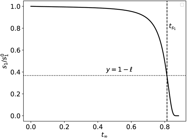
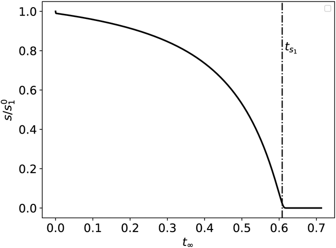
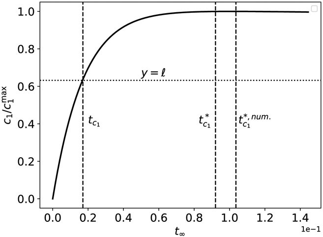
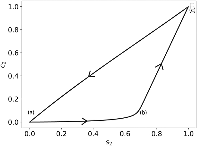
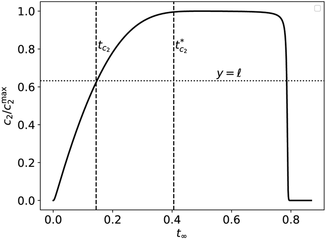
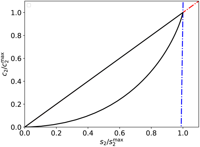
Scaling analysis exploiting timescale separation has been one of the most important techniques in the quantitative analysis of nonlinear dynamical systems in mathematical and theoretical biology. In the case of enzyme catalyzed reactions, it is often overlooked that the characteristic timescales used for the scaling the rate equations are not ideal for determining when concentrations and reaction rates reach their maximum values. In this work, we first illustrate this point by considering the classic example of the single-enzyme, single-substrate Michaelis-Menten reaction mechanism. We then extend this analysis to a more complicated reaction mechanism, the auxiliary enzyme reaction, in which a substrate is converted to product in two sequential enzyme-catalyzed reactions. In this case, depending on the ordering of the relevant timescales, several dynamic regimes can emerge. In addition to the characteristic timescales for these regimes, we derive matching timescales that determine (approximately) when the transitions from transient to quasi-steady-state kinetics occurs. The approach presented here is applicable to a wide range of singular perturbation problems in nonlinear dynamical systems.

Keywords: Chemical kinetics; Enzyme kinetics; Nonlinear dynamical systems; Perturbation methods; Slow and fast dynamics; Timescales.

Figure 1:. The validity of t_c1 for the Michaelis-Menten reaction mechanism (12).

The solid black curve is the numerically-computed solution to (13a)–(13b). The dashed vertical curve is corresponds to $t_{c_1}=[k_1(K_{M_1}+s_1^0){]}^{-1}$. The dotted horizontal line corresponds to $\ell c_1∕c_1^{\max }=\ell$. The initial concentrations and rate constants used in the numerical simulation are: k₁ = 0.1, k₂ = 10, k₋₁ = 1, $e_1^0=1$ and $s_1^0=100$ (units have been omitted). Time has been mapped to the t_∞ scale: t_∞(t) = 1 – 1/ln[t + exp(1)].

Figure 2:. The graphical illustration of the characteristic timescale for the Michaelis–Menten reaction mechanism (12).

When σ₁ ≪ 1, the timescale t_s1 is the characteristic time of the substrate species. The solid black curve is the numerical solution to the mass action equations (13a)–(13b) and the vertical dashed/dotted line corresponds to t = t_s1. The dotted horizontal line corresponds to the scaled characteristic value $(1-\ell )s_1^0$. The constants (without units) used in the numerical simulation are: $e_1^0=1$, k₁ = 0.01, k₂ = 10, k₋₁ = 1 and $s_1^0=100$. Time has been mapped to the t_∞ scale: t_∞(t) = 1 – 1/ln[t + exp(1)].

Figure 3:. The graphical illustrations of the completion timescale for the Michaelis–Menten reaction mechanism (12).

When σ₁ ≫ 1, the reaction is essentially complete when t = t_s1. The solid black curve is the numerical solution to the mass action equations (13a)–(13b) and the vertical dashed/dotted line corresponds to t = t_s1. The constants (without units) used in the numerical simulation are: $e_1^0=1$, k₁ = 10, k₂ = 10, k₋₁ = 1 and $s_1^0=100$. Time has been mapped to the t_∞ scale: t_∞(t) = 1 – 1/ln[t + exp(1)].

Figure 4:. A graphical comparison of the composite and numerical solutions for the time course of the Michaelis–Menten reaction (12).

The solid black curve is the numerical solution to (13a)–(13b). The unfilled circles mark the composite solution (33). The initial concentrations and rate constants used in the numerical simulation are: k₁ = 1, k₂ = 1, k₋₁ = 1, $e_1^0=1$ and $s_1^0=100$ (units have been omitted). All approximations have been scaled by their numerically-obtained maximum values, and time has been mapped to the t_∞ scale: t_∞(t) = 1 – 1/ln[t + exp(1)].

Figure 5:. The validity of tc1∗ and a graphical representation of its comparison with t_c1 for the Michaelis–Menten reaction mechanism (12).

The solid black curve is the numerically-computed solution to (13a)–(13b). The left-most dashed vertical curve is corresponds to t_c1, and the middle dashed vertical curve corresponds to the estimated value $t_{c_1}^{\ast }=-t_{c_1}\text{ln}{\epsilon }_2$. The dashed vertical line corresponds to the numerically-computed $t_{c_2}^{\ast }$, which is labeled as $t_{c_1}^{\ast ,num}$ in the figure. Notice that $t_{c_1}^{\ast }$ provides a much better estimate of the time it takes c₁ to reach its maximum than t_c1. The initial concentrations and rate constants used in the numerical simulation are: k₁ = 0.1, k₂ = 10, k₋₁ = 1, $e_1^0=1$ and $s_1^0=100$ (units have been omitted). Time has been mapped to the t_∞ scale: t_∞(t) = 1 – 1/ ln[t+exp(1)]. Note that the mass action equations have only been integrated from t = 0 to $t\approx t_{c_1}^{\ast }$ for clarity.

Figure 6:. The phase–plane portrait of the mass action trajectory for the auxiliary reaction mechanism (47)–(48).

The solid black curve is the numerically-computed solution to (49a)–(49d). The initial concentrations and rate constants used in the numerical simulation are: k₁ = 1, k₂ = 1, k₋₁ = 1, $e_1^0=1$, $e_2^0=100$, k₋₃ = 1, k₃ = 1, k₄ = 2 and $s_1^0=100$ (units have been omitted). s₂ and c₂ have been scaled by their numerically–obtained maximum values.

Figure 7:. The s₂–c₂ phase-plane trajectory (with nullclines) for the auxiliary reaction mechanism (47)–(48).

The thick black curve is the numerically-integrated solutions to the mass action equations (49a)–(49d). The broken red curve is the c₂-nullcline, and the broken blue curve is the fixed s₂-nullcline ($N_{s_2}^{\max }$, given by (56)). The phase–plane trajectory initially moves towards $N_{s_2}^{\max }$, then moves up $N_{s_2}^{\max }$ before moving back down the c₂-nullcline. The constants (without units) used in the numerical simulation are: $e_1^0=1$, $s_1^0=1000$, k₁ = 1, k₂ = 1, k₃ = 1, k₋₃ = 1, k₄ = 2, $e_2^0=100$ and k₋₁ = 1. Curves were scaled by their numerically obtained maximum values.

Figure 8:. A graphical illustration of the accuracy of the composite solutions for the auxiliary reaction mechanism (47)—(48).

The solid black curve is the numerical solution to (49c), and the unfilled circles mark the composite solution (84a). The constants (without units) used in the numerical simulation are: $e_1^0=1$, $s_1^0=1000$, $e_2^0=100$, k₁ = 1, k₂ = 1, k₃ = 1, k₋₃ = 1, k₄ = 2 and k₋₁ = 1. Time has been mapped to the t_∞ scale: t_∞(t) = 1 – 1/ln[t + exp(1)]. The substrate concentration has been scaled by its maximum value.

Figure 9:. The timescale t_c2 is characteristic of the time it takes c₂ to reach c2max, and the timescale tc2∗ is the approximate time it takes c₂ to reach c2max, respectively, in the auxiliary reaction mechanism (47)–(48).

The thick black curve is the numerically-integrated solutions to the mass action equations (49a)–(49d). The leftmost dashed vertical line corresponds to t_c2, and the rightmost dashed vertical line corresponds to $t_{c_2}^{\ast }=-t_{c_2}\text{ln}{t}_{c_2}∕t_{s_1}$. The lower dotted horizontal line corresponds to the scaled characteristic value $\ell c_2^{\max }$, and the upper dotted horizontal line corresponds to $c_2^{\max }$. The constants (without units) used in the numerical simulation are: $e_1^0=1$, $s_1^0=1000$, $e_2^0=100$, k₁ = 1, k₂ = 1, k₃ = 1, k₋₃ = 1, k₄ = 2 and k₋₁ = 1. Time has been mapped to the t_∞ scale: t_∞(t) = 1 – 1/ln[t + exp(1)], and c₂ has been numerically scaled by its maximum value. Note that the mass action equations have only been integrated from t = 0 to $t\approx t_{c_2}^{\ast }$ for clarity.

Figure 10:. The timescale t_s2 is characteristic of the time it takes s₂ to reach s2λ, and the timescale ts2∗ is the approximate time it takes s₂ to reach s2λ, respectively, in the auxiliary reaction mechanism (47)–(48).

The thick black curve is the numerically-integrated solution to the mass action equations (49a)–(49d). The leftmost dashed vertical line corresponds to t_s2, and the rightmost dashed vertical line corresponds to $t_{s_2}^{\ast }=-t_{s_2}\text{ln}{t}_{s_2}∕t_{c_2}$. The lower dotted horizontal line corresponds to the scaled characteristic value $\ell s_2^{\lambda }$, and the upper dashed/dotted vertical line corresponds to $s_2^{\lambda }$. The constants (without units) used in the numerical simulation are: $e_1^0=1$, $s_1^0=1000$, $e_2^0=100$, k₁ = 1, k₂ = 1, k₃ = 1, k₋₃ = 1, k₄ = 2 and k₋₁ = 1. Time has been mapped to the t_∞ scale: t_∞(t) = 1 – 1/ln[t + exp(1)], and s₂ has been numerically-scaled by its maximum value. For clarity, the mass action equations have been integrated from t = 0 to $t\approx t_{s_2}^{\ast }$.

Figure 11:. When t_c2, t_s2 ≪ t_c1, the timescale t_c1 is characteristic of the time it takes ṗ to reach its maximum, and the timescale tc1∗ is the approximate time it takes c₂ to reach its maximum, respectively, in the auxiliary reaction mechanism (47)–(48).

The thick black curve is the numerically-integrated solution to the mass action equations (49a)–(49d). The leftmost dashed vertical line corresponds to t_c1, and the rightmost dashed vertical line corresponds to $t_{c_1}^{\ast }=-t_{c_1}\text{ln}{t}_{c_1}∕t_{s_1}$. The lower dotted horizontal line corresponds to the scaled characteristic value $\ell s_2^{\lambda }$. The constants (without units) used in the numerical simulation are: $e_1^0=1$, $s_1^0=100$, $e_2^0=100$, k₁ = 0.01, k₂ = 1, k₃ = 10, k₋₃ = 1, k₄ = 100 and k₋₁ = 1. Time has been mapped to the t_∞ scale: t_∞(t) = 1 – 1/ln[t + exp(1)], and c₂ has been numerically scaled by its maximum value.

Figure 12:. No significant change in the concentration of s₂ or c₂ occurs over the timescale t_c2 in the auxiliary reaction mechanism (47)–(48) when t_c1 ≪ t_c2 ≪ t_s2 ≪ t_s1.

The thick black curve is the numerically-integrated solutions to the mass action equations (49a)–(49d). The dashed vertical line corresponds to t_c2 Note that there is no significant increase in the concentration of the intermediate complex over the t_c2 timescale. The constants (without units) used in the numerical simulation are: $e_1^0=1$, $s_1^0=1000$, $e_2^0=1$, k₁ = 1, k₂ = 1, k₃ = 1, k₋₃ = 1, k₄ = 100 and k₋₁ = 1. Time has been mapped to the t_∞ scale: t_∞(t) = 1 — 1/ln[t + exp(1)], and c₂ has been scaled its maximum value.

Figure 13:. The validity of ts2χ and ts2χ,∗ in the auxiliary reaction mechanism (47)–(48) when ϵ ≪ 1.

The thick black curve is the numerically-integrated solution to the mass action equations (49a)–(49d), and the unfilled circles mark the inner solution given by (103). The leftmost dashed vertical line corresponds to $t_{s_2}^{\chi }$, and the rightmost dashed vertical line corresponds to $t_{s_2}^{\chi ,\ast }=-t_{s_2}^{\chi }\text{ln}{t}_{s_2}^{\chi }∕t_{s_1}$. The lower dotted horizontal line corresponds to $y=\ell s_2^{\max }$, and the upper dotted horizontal line corresponds to $y=s_2^{\max }$. The constants (without units) used in the numerical simulation are: $e_1^0=1$, $s_1^0=1000$, $e_2^0=1$, k₁ = 1, k₂ = 1, k₃ = 1, k₋₃ = 1, k₄ = 100 and k₋₁ = 1. Time has been mapped to the t_∞ scale: t_∞(t) = 1 – 1/ln[t + exp(1)], and s₂ has been numerically-scaled by its maximum value. Note that the mass action equations have only been integrated from t = 0 to $t\approx t_{s_2}^{\chi ,\ast }$ for clarity.

Figure 14:. The lag time in the auxiliary reaction mechanism (47)–(48) when t_s2 ≪ t_c1 ≪ t_c2 ≪ t_s1.

The thick black curve is the numerically-integrated solution to the mass action equations (49a)–(49d), and the unfilled circles mark the inner solution given by (103). The leftmost dashed vertical line corresponds to t_c2, and the rightmost dashed vertical line corresponds to $t_{c_2}^{\ast }=-t_{c_2}\text{ln}{t}_{c_2}∕t_{s_1}$. The lower dotted horizontal line corresponds to y = ℓ; The constants (without units) used in the numerical simulation are: $e_1^0=1$, $s_1^0=1000$, $e_2^0=1$, k₁ = 1, k₂ = 1, k₃ = 1, k₋₃ = 1, k₄ = 100 and k₋₁ = 1. Time has been mapped to the t_∞ scale: t_∞(t) = 1 – 1/ln[t + exp(1)], and c₂ has been numerically-scaled by its maximum value.

Figure 15:. Phase–plane dynamics of the auxiliary reaction mechanism (47)— (48) when t_c1 ≪ t_c2 ≪ t_s2 ≪ t_s1.

The thick black curve is the numerically-integrated solution to the mass action equations (49a)–(49d), the dashed/dotted red curve is the c₂-nullcline and the dashed/dotted blue curve is the stationary s₂-nullcline. Notice that the trajectory does not follow a path that lies close to either nullcline in the approach to x*. The constants (without units) used in the numerical simulation are: $e_1^0=1$, $s_1^0=1000$, $e_2^0=10$, k₁ = 1, k₂ = 1, k₃ = 10, k₋₃ = 1, k₄ = 100 and k₋₁ = 1.

Figure 16:. The lag time in the auxiliary reaction mechanism (47)–(48) when t_c1 ≪ t_c2 = t_s2 ≪ t_s1.

This is a close-up of Figure 15 near x*. The thick black curve is the numerically-integrated solution to the mass action equations (49a)–(49d), the dashed/dotted red curve is the c₂-nullcline and the dashed/dotted blue curve is the stationary s₂-nullcline. The solid black circle marks the trajectory when $t=t_{s_2}^{\ast }=-t_{s_2}\text{ln}{t}_{s_2}∕t_{s_1}$. Notice that Tikhonov’s Theorem still provides a reasonable estimate of the lag time, which is synonymous with the matching timescale corresponding to either s₂ or c₂. The constants (without units) used in the numerical simulation are: $e_1^0=1$, $s_1^0=1000$, $e_2^0=10$, k₁ = 1, k₂ = 1, k₃ = 10, k₋₃ = 1, k₄ = 100 and k₋₁ = 1.

Figure 17:. The trajectory follows the s₂-nullcline in the phase–plane of the auxiliary reaction mechanism (47)-(48) when ts2χ∕ts1≪1.

The thick black curve is the numerically-integrated solution to the mass action equations (49a)–(49d), the dashed/dotted red curve is the c₂-nullcline and the dashed/dotted blue curve is a snapshot of s₂-nullcline when t ≈ 1.1 · t_s1. The black dot is the corresponding snapshot of the numerical solution to (49a)–(49d). In this simulation, $t_{s_2}^{\chi }∕t_{s_1}\approx 0.001<{\mu }_2\approx 0.1$; consequently, the trajectory follows the s₂-nullcline but fails to closely follow x* (see Movie 1 in Supplementary Materials). The constants (without units) used in the numerical simulation are: $e_1^0=1$, $s_1^0=100$, $e_2^0=100$, k₁ = 1, k₂ = 1, k₃ = 1, k₋₃ = 1, k₄ = 0.1 and k₋₁ = 1.

Figure 18:. The component-wise error when the indicator reaction is fast in the auxiliary reaction mechanism (47)–(48).

The thick black curve is the numerically-integrated solution to the mass action equations (49a)–(49d), the dashed/dotted red curve is the c₂-nullcline and the dashed/dotted blue curve is a snapshot of s₂-nullcline when t ≈ 1.1 · t_s1. The black dot is the corresponding snapshot of the numerical solution to (49a)–(49d). In this simulation, $t_{s_2}^{\chi }∕t_{s_1}\approx 0.0001<{\mu }_2\approx 0.005$; consequently, the trajectory sits “just behind” and slightly above x* (green dot) since the trajectory will be closer to the s₂-nullcline than the c₂-nullcline (see Movie 2 in Supplementary Materials). The constants (without units) used in the numerical simulation are: $e_1^0=1$, $s_1^0=100$, $e_2^0=100$, k₁ = 1, k₂ = 1, k₃ = 1, k₋₃ = 1, k₄ = 2 and k₋₀ = 1.

References

1. Berglund N, Gentz B, 2006. Noise-induced phenomena in slow-fast dynamical systems. Springer-Verlag London, Ltd., London.
1. Bersani AM, Bersani E, Dell’Acqua G, Pedersen MG, 2015. New trends and perspectives in nonlinear intracellular dynamics: one century from Michaelis-Menten paper. Contin. Mech. Thermodyn 27, 659–684.
1. Bersani AM, Dell’Acqua G, 2012. Is there anything left to say on enzyme kinetic constants and quasi-steady state approximation? J. Math. Chem 50, 335–344.
1. Bertram R, Rubin JE, 2017. Multi-timescale systems and fast-slow analysis. Math. Biosci 287, 105–121. - PubMed
1. Borghans JAM, Boer RJD, Segel LA, 1996. Extending the quasi-steady state approximation by changing variables. Bull. Math. Biol 58, 43–63. - PubMed
Publication types
LinkOut - more resources