Multimodal Modeling of Neural Network Activity: Computing LFP, ECoG, EEG, and MEG Signals With LFPy 2.0

Abstract

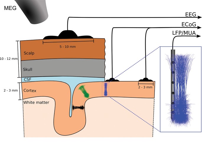
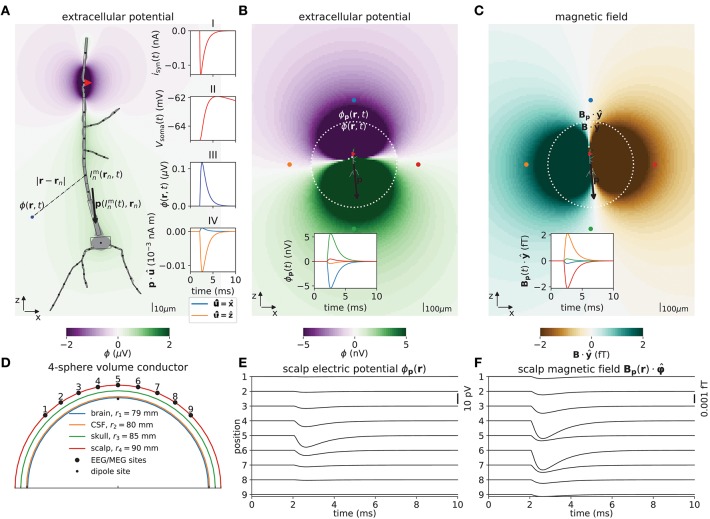
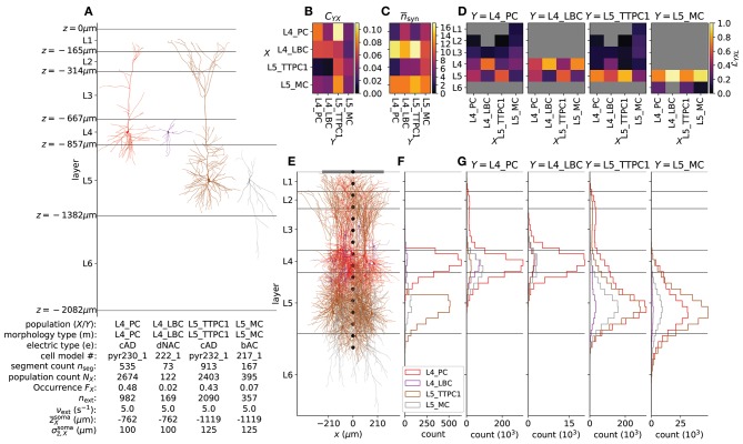
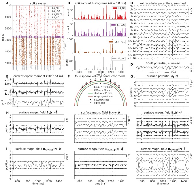
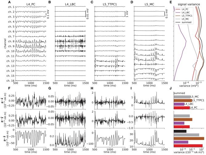
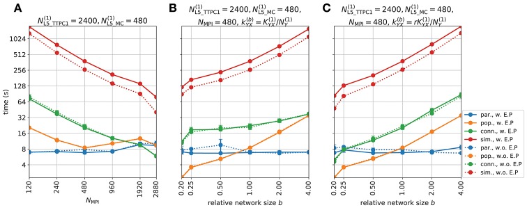
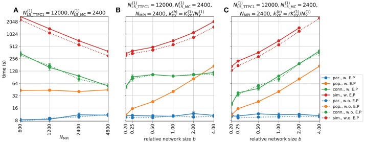
Recordings of extracellular electrical, and later also magnetic, brain signals have been the dominant technique for measuring brain activity for decades. The interpretation of such signals is however nontrivial, as the measured signals result from both local and distant neuronal activity. In volume-conductor theory the extracellular potentials can be calculated from a distance-weighted sum of contributions from transmembrane currents of neurons. Given the same transmembrane currents, the contributions to the magnetic field recorded both inside and outside the brain can also be computed. This allows for the development of computational tools implementing forward models grounded in the biophysics underlying electrical and magnetic measurement modalities. LFPy (LFPy.readthedocs.io) incorporated a well-established scheme for predicting extracellular potentials of individual neurons with arbitrary levels of biological detail. It relies on NEURON (neuron.yale.edu) to compute transmembrane currents of multicompartment neurons which is then used in combination with an electrostatic forward model. Its functionality is now extended to allow for modeling of networks of multicompartment neurons with concurrent calculations of extracellular potentials and current dipole moments. The current dipole moments are then, in combination with suitable volume-conductor head models, used to compute non-invasive measures of neuronal activity, like scalp potentials (electroencephalographic recordings; EEG) and magnetic fields outside the head (magnetoencephalographic recordings; MEG). One such built-in head model is the four-sphere head model incorporating the different electric conductivities of brain, cerebrospinal fluid, skull and scalp. We demonstrate the new functionality of the software by constructing a network of biophysically detailed multicompartment neuron models from the Neocortical Microcircuit Collaboration (NMC) Portal (bbp.epfl.ch/nmc-portal) with corresponding statistics of connections and synapses, and compute in vivo-like extracellular potentials (local field potentials, LFP; electrocorticographical signals, ECoG) and corresponding current dipole moments. From the current dipole moments we estimate corresponding EEG and MEG signals using the four-sphere head model. We also show strong scaling performance of LFPy with different numbers of message-passing interface (MPI) processes, and for different network sizes with different density of connections. The open-source software LFPy is equally suitable for execution on laptops and in parallel on high-performance computing (HPC) facilities and is publicly available on GitHub.com.

Keywords: ECoG; EEG; LFP; MEG; local field potential; modeling; neuron; neuronal network.

Figure 1

Illustration of measurement signals computed by LFPy 2.0. The figure illustrates the EEG, ECoG, LFP/MUA (linear multielectrode) and MEG recordings of electrical and magnetic signals stemming from populations of cortical neurons. Here three separate cortical populations are depicted. EEG electrodes are placed on the scalp, ECoG electrodes on the cortical surface, while the LFP and MUA both are recorded by electrodes placed inside cortex. In MEG the tiny magnetic fields stemming from brain activity is measured by SQUIDs placed outside the head. The MUA signal, that is, the high-frequency part of the recorded extracellular potential inside cortex, measures spikes from neurons in the immediate vicinity of the electrode contact, typically less than 100 μm away (Buzsáki, ; Pettersen and Einevoll, ; Pettersen et al., 2008). The “mesoscopic” LFP and ECoG signals will typically contain information from neurons within a few hundred micrometers or millimeters from the recording contact (Einevoll et al., 2013), while the “macroscopic” EEG and MEG signals will have contributions from cortical populations even further away (Hämäläinen et al., ; Nunez and Srinivasan, 2006).

Figure 2

Illustrations of forward model, dipole approximation, EEG and MEG model. (A) Illustration of forward-modeling scheme for extracellular potentials from multicompartment neuron models. The gray shape illustrates soma and dendrites of a 3D-reconstructed neuron morphology and the equivalent multicompartment model. A single synaptic input current i_syn(t) (red triangle, inset axes I) results in a deflection of the membrane voltage throughout the morphology, including at the soma (V_soma(t), inset axes II). LFPy allows for computing extracellular potentials ϕ in arbitrarily chosen extracellular locations r (inset axes III) from transmembrane currents ($I_n^{\text{m}}({\text{r}}_n,t)$), as well as the components of the current dipole moment p (black arrow, inset axes IV). Compartments are indexed n, r_n denote compartment positions. The image plot shows the extracellular potential in the xz-plane at the time of the largest synapse current magnitude (t = 2.25 ms). (B) Illustration of the extracellular electric potential calculated both from the current dipole moment and transmembrane currents for the situation in (A). Within a radius r < 500 μm from the “center of areas” (see below) of the morphology the panel shows extracellular potentials ϕ(r) predicted using the line-source method, while outside this radius the panel shows extracellular potentials ϕ_p(r) predicted from the current dipole moment (p, black arrow). Here, an assumption of an homogeneous (same everywhere) and isotropic (same in all directions) extracellular conductivity was used. The ‘center of areas‘ was defined as $\sum _{n=1}^{n^{\text{seg}}}{A}_n{\text{r}}_n/\sum _{n=1}^{n^{\text{seg}}}{A}_n$ where A_n denotes compartment surface area. The time t = 2.25 ms as in (A). The inset axis shows the potential as function of time in the four corresponding locations (at |R| = 750 μm) surrounding the morphology (colored circular markers). (C) Visualization of magnetic field component ${\text{B}}_{\text{p}}·\widehat{\text{y}}$ (y-component) computed from the current dipole moment, outside a circle of radius r = 500 μm (as in B). Inside the circle, we computed the same magnetic field component from axial currents. The inset axis shows the y-component of the magnetic field as function of time in the four corresponding locations (at |R| = 750 μm) surrounding the morphology (circular markers). (D) Illustration of upper half of the four-sphere head model used for predictions of EEG scalp potentials from electric current dipole moments. Each spherical shell with outer radii r ∈ {r₁, r₂, r₃, r₄} has piecewise homogeneous and isotropic conductivity σ_e ∈ {σ₁, σ₂, σ₃, σ₄}. The EEG/MEG sites numbered 1–9 mark the locations where electric potentials and magnetic fields are computed, each offset by an arc length of r₄π/16 in the xz-plane. The current dipole position was θ = φ = 0, r = 78 mm (in spherical coordinates). (E) Electric potentials on the outer scalp-layer positions 1-9 in (D). (F) Tangential component of the magnetic field ${\text{B}}_{\text{p}}·\widehat{\phi }$ in positions 1–9. (Note that at position 5, the unit vector $\widehat{\phi }$ is defined to be directed in the positive y-direction).

Figure 3

Axial currents in multicompartment neuron models. (A) Schematic illustration of sections (colored rectangles), segments and equivalent electric circuit of a simplified multicompartment neuron model. The relative length χ varies between 0 and 1 from start- to end-point of each section. (B) Axial current line element vectors (d_m, d_m+1) and corresponding midpoints (r_m, r_m+1) of axial currents ($I_m^{\text{a}},I_{m+1}^{\text{a}}$) between two connected segments. (C) Axial currents ($I_m^{\text{a}},I_{m+1}^{\text{a}}$), membrane potentials ($V_f^{\text{m}},V_n^{\text{m}}$), and axial resistance ($R_{fn}^{\text{i}}$) in equivalent electric circuit for a parent segment f and child segment n in a single section. (D) Similar to panel B, but parent and child segments belong to two different sections. The total series resistance is here $R_f^{\text{i}}+R_n^{\text{i}}$. (E) Illustration of the case where the child segment n is connected to a point χ = 0.5 on the parent section. For children connected at χ ∈ 〈0, 1〉 the voltage difference ($V_n^{\text{m}}-V_f^{\text{m}}$) is only across the child segment axial resistance $R_n^{\text{i}}$, but the (virtual) current from the node connecting the child start point to the parent midpoint $I_m^{\text{a}}$ is still accounted for. (F) Illustration of axial currents at branch point between different sections of the morphology. The child segment n has one parent f and one sibling indexed by ñ, where $V_{\times }^{\text{m}}$ denotes the virtual membrane potential at the node connecting the parent end-point to the children start-points. $V_{ñ}^{\text{m}}$ is the voltage in the midpoint of the sibling segment, while $R_{ñ}^{\text{i}}$ and $I_{\tilde{m}}^{\text{a}}$ denotes the axial resistance and current between the sibling midpoint and the branch point.

Figure 4

Details of the example network. (A) Biophysically detailed neuron models of the network, with depth-values of boundaries of layers 1–6. The lower left table summarizes population names (X – presynaptic; Y – postsynaptic) which here coincide with morphology type (m); electric type (e); cell model #; compartment count per single-cell model ($n_j^{\text{seg}}$); number of cells N_X in each population; occurrence F_X (defined as $N_X/\sum _X{N}_X$); the number of external synapses on each cell n_ext; rate expectation of external synapses ν_ext; the expected mean ${\overline{z}}_X^{\text{soma}}$ and standard deviation ${\sigma }_{\overline{z},X}^{\text{soma}}$ of the normal distribution $\mathcal{N}$ from which somatic depths are drawn. (B) Pairwise connection probability C_YX between cells in presynaptic populations X and postsynaptic populations Y. (C) Average number ${\overline{n}}^{\text{syn}}$ of synapses created per connection between X and Y. (D) Layer specificity of connections ${\mathcal{L}}_{YXL}$ (Hagen et al., 2016) from each presynaptic population X onto each postsynaptic population Y. Gray values denote ${\mathcal{L}}_{YXL}=0$. (E) Illustration of cylindrical geometry of populations including a laminar recording device for extracellular potentials (black circular markers) and a single ECoG electrode above layer 1 (gray line). n = 15 neurons of each population are shown in their respective locations. (F) Laminar distribution of somas for each network population (Δz = 50 μm) in one instantiation of the circuit. (G) Laminar distribution of synapses across depth onto each postsynaptic population Y from presynaptic populations X (Δz = 50 μm).

Figure 5

Intra- and extracellular measures of activity in example network. (A) Spike raster plot for each population. Each row of dots corresponds to the spike train of one neuron, color coded by population. (B) Population spike rates computed by summing number of spike events in each population in temporal bins of width Δt = 5 ms. (C) Extracellular potentials as function of depth assuming an infinite volume conductor. (D) Extracellular potential on top of cortex (ECoG) assuming a discontinuous jump in conductivity between brain (σ = 0.3 S/m) and a non-conducting cover medium (σ = 0 S/m) and electrode surface radius r = 250 μm. The signal is compared to the channel 1 extracellular potential in (C) (gray line). (E) Component-wise contributions to the total current dipole moment p(t) summed over population contributions. (F) Illustration of upper half of the four-sphere head model (with conductivities σ_s ∈ {0.3, 1.5, 0.015, 0.3} S/m and radii r_s ∈ {79, 80, 85, 90} mm for brain, csf, skull and scalp, respectively), dipole location in inner brain sphere and scalp measurement locations. The sites in the xz-plane numbered 1–9 mark the locations where electric potentials and magnetic fields are computed, each offset by an arc length of r₄π/16 ≈ 18 mm. (G) EEG scalp potentials from multicompartment-neuron network activity with radially oriented populations. (H) Tangential and radial components of the head-surface magnetic field (MEG) from multicompartment-neuron network activity with radially oriented population. (I) Tangential and radial components of the magnetic field (MEG) on the head surface, with underlying dipole sources rotated by an angle θ = π/2 around the x-axis (thus with apical dendrites pointing into the plane). (Note that at position 5, the unit vectors $\widehat{\phi }$ and $\widehat{\theta }$ are defined to be directed in the positive y- and x-directions, respectively).

Figure 6

Per-population contributions to the extracellular potential and current dipole moment and corresponding signal variance. (A–D) Contributions to the extracellular potential from populations X ∈ {L4_PC, L4_LBC, L5_TTPC1, L5_MC} in the network across depth. (E) Extracellular potential variance across depth for contributions of each population, and for the sum over populations. (F–I) x, y, z-components of the per-population contribution to the summed current dipole moment. (J) Per-component current dipole moment variance for each population and for summed signals.

Figure 7

Parallel performance with networks in LFPy. (A) Initialization of parameters (par.), population create (pop.), connectivity build (conn.) and main simulation time (sim.) as functions of number of physical CPU cores/MPI processes (N_MPI). The reference network population sizes $N_X^{(1)}$ for X ∈ {L5_TTPC1, L5_MC} are given in the panel title. The network was otherwise constructed with synapse, stimulus and connectivity parameters for each possible connection as given in Tables 1–3. Times shown with continuous lines were obtained for simulations that included calculations of extracellular potentials and current dipole moments as in Figures 2–6 (w. E.P.), while times shown with dotted lines were obtained for simulations with no such signal predictions (w.o. E.P.). Each data value is shown as the mean and standard deviation of times obtained from N = 3 network realizations instantiated with different random seeds. (B) Initialization of parameters, population create, connectivity build and main simulation time as functions of network size relative to the reference network population sizes $N_X^{(1)}$ for X ∈ {L5_TTPC1, L5_MC} as given in the panel title. The superset “(1)” denotes a relative network size b = 1. Simulations were run using a fixed MPI process count N_MPI and connection probabilities $C_{YX}^{(r)}$ were recomputed for different values of b, such that the expected total number of connections $K_{YX}^{(1)}$ was constant between each simulation (using 20). The set-up was otherwise identical to the set-up in (A). (C) Same as (B), but with a fixed expected per-cell synapse in-degree $k_{YX}^{(r)}\equiv r{K}_{YX}^{(1)}/N_Y^{(1)}$ across different relative network sizes.

Figure 8

Parallel performance with networks in LFPy II. (A) Similar to Figure 7A, but with network population sizes upscaled by a factor 5, and a corresponding increase in parallel job sizes. (B,C) Similar to Figures 7B,C, but with network population sizes and parallel job sizes increased by a factor 5.

References

1. Abdellah M., Bilgili A., Eilemann S., Markram H., Schürmann F. (2015). Physically-based in silico light sheet microscopy for visualizing fluorescent brain models. BMC Bioinformatics 16:S8. 10.1186/1471-2105-16-S11-S8 - DOI - PMC - PubMed
1. Abdellah M., Bilgili A., Eilemann S., Shillcock J., Markram H., Schürmann F. (2017). Bio-physically plausible visualization of highly scattering fluorescent neocortical models for in silico experimentation. BMC Bioinformatics 18:62. 10.1186/s12859-016-1444-4 - DOI - PMC - PubMed
1. Almog M., Korngreen A. (2014). A quantitative description of dendritic conductances and its application to dendritic excitation in layer 5 pyramidal neurons. J. Neurosci. 34, 182–196. 10.1523/JNEUROSCI.2896-13.2014 - DOI - PMC - PubMed
1. Anastassiou C. A., Perin R., Markram H., Koch C. (2011). Ephaptic coupling of cortical neurons. Nat. Neurosci. 14, 217–223. 10.1038/nn.2727 - DOI - PubMed
1. Bangera N. B., Schomer D. L., Dehghani N., Ulbert I., Cash S., Papavasiliou S., et al. (2010). Experimental validation of the influence of white matter anisotropy on the intracranial EEG forward solution. J. Comput. Neurosci. 29, 371–387. 10.1007/s10827-009-0205-z - DOI - PMC - PubMed
LinkOut - more resources