. 2019 Jan 14;9(1):111.
doi: 10.1038/s41598-018-36816-z.

Slow insertion of silicon probes improves the quality of acute neuronal recordings

Affiliations

Slow insertion of silicon probes improves the quality of acute neuronal recordings

Richárd Fiáth et al. Sci Rep. .

Abstract

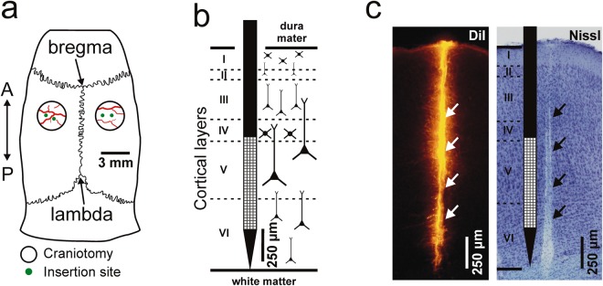
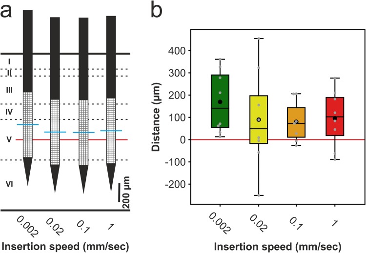
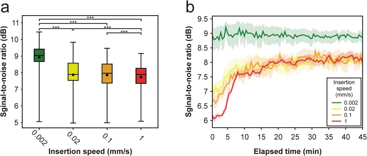
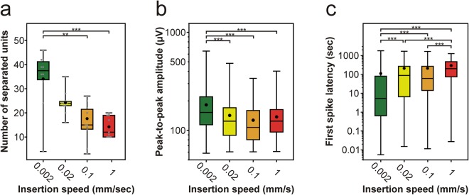
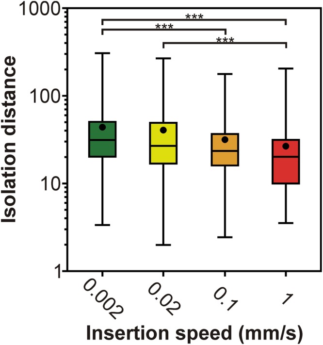
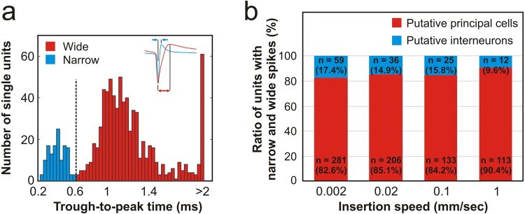
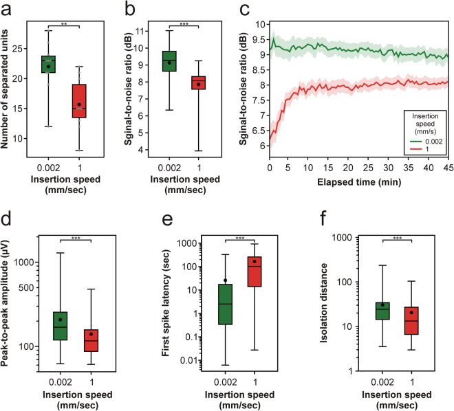
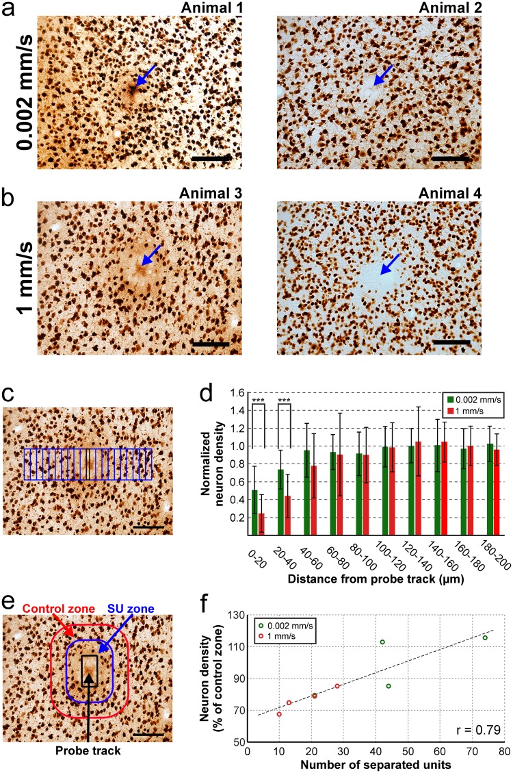
Neural probes designed for extracellular recording of brain electrical activity are traditionally implanted with an insertion speed between 1 µm/s and 1 mm/s into the brain tissue. Although the physical effects of insertion speed on the tissue are well studied, there is a lack of research investigating how the quality of the acquired electrophysiological signal depends on the speed of probe insertion. In this study, we used four different insertion speeds (0.002 mm/s, 0.02 mm/s, 0.1 mm/s, 1 mm/s) to implant high-density silicon probes into deep layers of the somatosensory cortex of ketamine/xylazine anesthetized rats. After implantation, various qualitative and quantitative properties of the recorded cortical activity were compared across different speeds in an acute manner. Our results demonstrate that after the slowest insertion both the signal-to-noise ratio and the number of separable single units were significantly higher compared with those measured after inserting probes at faster speeds. Furthermore, the amplitude of recorded spikes as well as the quality of single unit clusters showed similar speed-dependent differences. Post hoc quantification of the neuronal density around the probe track showed a significantly higher number of NeuN-labelled cells after the slowest insertion compared with the fastest insertion. Our findings suggest that advancing rigid probes slowly (~1 µm/s) into the brain tissue might result in less tissue damage, and thus in neuronal recordings of improved quality compared with measurements obtained after inserting probes with higher speeds.


Conflict of interest statement

The authors declare no competing interests.

Figures

Figure 1
Figure 1
Schematic illustration of the experimental design. (a) The position of the four insertion sites (green dots) of a representative experiment shown on the schematic of a rat skull. The two craniotomies (hollow black circles) were prepared over the trunk region of the primary somatosensory cortex (A, anterior; P, posterior). (b) Schematic demonstration of the approximate position of the high-density silicon probe in the brain tissue after inserting it to a dorsoventral depth of 1700 µm. Small white squares mark the recording sites. Boundaries between cortical layers (roman numerals) are indicated with dashed lines. Note that most of the recording sites were located in layer V. (c) Representative coronal brain section prepared from the right brain hemisphere. On the left, fluorescent marks of DiI are visible indicating the track of the probe. On the right, the same brain section after Nissl-staining. Arrows indicate the position of the probe track, while dashed lines mark cortical layer boundaries.
Figure 2
Figure 2
Estimated position of the recording sites relative to cortical layer V for each insertion speed. (a) The average distance between the depth corresponding to the middle of layer V (red line) and the depth corresponding to the middle of the electrode array (blue line) for each insertion speed. The depth of the insertion as well as the location of layer V was estimated by examining the coronal brain sections. Cortical layers are indicated with roman numerals. (b) Box-and-whisker plot of the distances between the middle of layer V (red line) and the middle of the electrode array for each insertion speed. On the box-and-whisker plot, the middle line indicates the median, while the boxes correspond to the 25th and 75th percentile. Whiskers mark the minimum and maximum values. The average is depicted with a black dot. Gray dots correspond to distance values obtained for individual penetrations (8 penetrations for speeds: 0.002 mm/s, 0.02 mm/s and 1 mm/s; 7 penetrations for speed: 0.1 mm/s). The distance values were not significant between insertion speeds (one-way ANOVA; p = 0.656).
Figure 3
Figure 3
Quality of neuronal recordings after the slowest (0.002 mm/s) and the fastest (1 mm/s) probe insertion. (a) Schematic of the tip section of the silicon probe comprising 128 close-packed electrodes (white and black squares), with the electrode–channel relationship indicated (red text; Ch, channel). Representative three-second-long multi-unit activity (MUA) traces recorded after slow (b) and after fast (c) insertion on eight electrodes (colored black in panel (a)). Traces on the left show MUA shortly after probe insertion (1st min), while traces on the right were obtained 45 minutes after implantation (45th min). The same voltage scale was used on all the traces. Color maps constructed from three-second-long data recorded on all channels after slow (d) and after fast (e) insertion. Color maps on the left show MUA shortly after probe insertion (1st min), while color maps on the right were constructed from data recorded 45 minutes after implantation (45th min). Before plotting the color maps, the absolute value of the MUA was calculated, then a 30 Hz low-pass filter was applied on the data to obtain the envelope of the MUA (au; arbitrary unit). Black traces below the color maps show the instantaneous population activity recorded by the probe at each sample point of the three seconds, which was obtained by summing the values on all of the channels.
Figure 4
Figure 4
Neuronal activity obtained after probe insertion with the slowest speeds showed the highest and most stable signal-to-noise ratio. (a) Box-and-whisker plot of the signal-to-noise ratio (SNR) values for each insertion speed. SNR values were calculated from consecutive, 30-second-long segments of the recordings, during the entire 45-minute-long recording period, then averaged across channels (number of computed SNR values after data cleansing for each speed: 0.002 mm/s, n = 897; 0.02 mm/s, n = 867; 0.1 mm/s, n = 802; 1 mm/s, n = 753). On the box-and-whisker plot, the middle line indicates the median, while the boxes correspond to the 25th and 75th percentile. Whiskers mark the minimum and maximum values. The average is depicted with a black dot. ***p < 0.001; Dunn’s post-hoc test with Bonferroni correction. (b) Change in the average SNR of the recorded spiking activity over time for each insertion speed. Colored bands correspond to the standard error of mean.
Figure 5
Figure 5
Insertion speed-dependent difference in the properties of the recorded single-unit activity. (ac) Box-and-whisker plots showing the distribution of the number of well-separated single unit clusters (a), the distribution of the peak-to-peak amplitude of spike waveforms (b), and the distribution of the first spike latencies (c) for each insertion speed (total number of well-separated neurons for each speed: 0.002 mm/s, n = 341; 0.02 mm/s, n = 242; 0.1 mm/s, n = 159; 1 mm/s, n = 128). On the box-and-whisker plots, the middle line indicates the median, while the boxes correspond to the 25th and 75th percentile. Whiskers mark the minimum and maximum values. The average is depicted with a black dot. Gray dots on panel (a) correspond to single unit yields obtained for individual penetrations. Data on panel (b) and (c) are plotted on a logarithmic scale. **p < 0.01; ***p < 0.001; Dunn’s post-hoc test with Bonferroni correction.
Figure 6
Figure 6
Insertion speed-dependent difference in the quality of single unit clusters. Box-and-whisker plots showing the distribution of the isolation distance of well-separated single unit clusters for each insertion speed (total number of well-separated neurons for each speed: 0.002 mm/s, n = 341; 0.02 mm/s, n = 242; 0.1 mm/s, n = 159; 1 mm/s, n = 128). On the box-and-whisker plots, the middle line indicates the median, while the boxes correspond to the 25th and 75th percentile. Whiskers mark the minimum and maximum values. The average is depicted with a black dot. Data are plotted on a logarithmic scale. ***p < 0.001; Dunn’s post-hoc test with Bonferroni correction.
Figure 7
Figure 7
Ratio of putative interneurons and principal cells among insertion speeds. (a) Bimodal distribution of the trough-to-peak time of single unit spike waveforms. A threshold of 0.6 ms (vertical dashed line) was used to classify units either as narrow spiking (blue) or as wide spiking (red) neurons (i.e. as putative inhibitory interneurons or excitatory principal cells, respectively). A sample average spike waveform of each neuron type is shown in the inset. (b) Ratio of putative principal cells (wide spikes, red) and putative interneurons (narrow spikes, blue) calculated for each insertion speed. The number of neurons in each group is indicated.
Figure 8
Figure 8
Quality of neuronal recordings after inserting the 15-µm-thick, 32-channel silicon probe with the slowest (0.002 mm/s) and the fastest (1 mm/s) speed. (a) Schematic of the tip section of the silicon probe comprising 32 electrodes (white and black squares), with the electrode–channel relationship indicated (red text; Ch, channel). Representative three-second-long multi-unit activity (MUA) traces recorded after slow (b) and after fast (c) insertion on eight electrodes (colored black in panel (a)). Traces on the left show MUA shortly after probe insertion (1st min), while traces on the right were obtained 45 minutes after implantation (45th min). The same voltage scale was used on all the traces. Color maps constructed from three-second-long data recorded on all channels after slow (d) and after fast (e) insertion. Color maps on the left show MUA shortly after probe insertion (1st min), while color maps on the right were constructed from data recorded 45 minutes after implantation (45th min). Before plotting the color maps, the absolute value of the MUA was calculated, then a 30 Hz low-pass filter was applied on the data to obtain the envelope of the MUA (au; arbitrary unit). Black traces below the color maps show the instantaneous population activity recorded by the probe at each sample point of the three seconds, which was obtained by summing the values on all of the channels.
Figure 9
Figure 9
Insertion speed-dependent difference in the properties of the single-unit activity recorded with the 32-channel silicon probe. (a) Box-and-whisker plot showing the distribution of the number of well-separated single unit clusters. (b) Box-and-whisker plot of the signal-to-noise ratio (SNR) values for each insertion speed. SNR values were calculated from consecutive, 30-second-long segments of the recordings, during the entire 45-minute-long recording period, then averaged across channels (number of computed SNR values after data cleansing for each speed: 0.002 mm/s, n = 899; 1 mm/s, n = 896). (c) Change in the average SNR of the recorded spiking activity over time for each insertion speed. Colored bands correspond to the standard error of mean. (df) Box-and-whisker plot showing the distribution of the peak-to-peak amplitude of spike waveforms (d), the distribution of the first spike latencies (e), and the distribution of the isolation distances (f) for each insertion speed (total number of well-separated neurons for each speed: 0.002 mm/s, n = 220; 1 mm/s, n = 157). On the box-and-whisker plots, the middle line indicates the median, while the boxes correspond to the 25th and 75th percentile. Whiskers mark the minimum and maximum values. The average is depicted with a black dot. Gray dots on panel (a) correspond to single unit yields obtained for individual penetrations. Data on panels (d-f) are plotted on a logarithmic scale. **p < 0.01; ***p < 0.001; Mann-Whitney U test.
Figure 10
Figure 10
Insertion speed-dependent difference in the neuronal cell loss around the probe track. (a,b) Representative NeuN-stained horizontal brain sections showing the probe track (blue arrow) and nearby neurons (small dark patches) after penetrations done either with the slowest (a) or with the fastest (b) insertion speed. Brain sections from two animals are shown for each speed. 20-fold magnification. Scale bars = 100 µm. (c) Neuron numbers were automatically counted in twenty bins (blue rectangles having an area of 20 × 100 µm2) on each side of the probe track (black rectangle in the center; area: 10 × 100 µm2). Only ten bins are shown on each side. Scale bar = 100 µm. (d) Normalized neuron density in the first ten 20-µm-wide bin located closest to the probe track for each insertion speed after automatic image analysis. Average and standard deviation is presented. Normalized neuron densities were averaged across penetrations and sides. ***p < 0.001; Student’s t-test. (e) To complement the results of the automatic cell counting, neuron numbers were manually counted in two zones around the probe track (black rectangle). The single unit (SU) zone was located 0–50 µm from the probe track (blue rounded rectangle), while the control zone was 50–100 µm away from the track (red rounded rectangle). Scale bar = 100 µm. Neuron density measured in the SU zone was normalized to the neuron density in the control zone. (f) Scatter plot showing a strong correlation between the single unit yield and the normalized neuron density in the SU zone.

Similar articles

Cited by

References

    1. Buzsáki G. Large-scale recording of neuronal ensembles. Nat. Neurosci. 2004;7:446–451. doi: 10.1038/nn1233. - DOI - PubMed
    1. Fiáth R, et al. A silicon-based neural probe with densely-packed low-impedance titanium nitride microelectrodes for ultrahigh-resolution in vivo recordings. Biosens. Bioelectron. 2018;106:86–92. doi: 10.1016/j.bios.2018.01.060. - DOI - PubMed
    1. Jun JJ, et al. Fully integrated silicon probes for high-density recording of neural activity. Nature. 2017;551:232–236. doi: 10.1038/nature24636. - DOI - PMC - PubMed
    1. Raducanu BC, et al. Time Multiplexed Active Neural Probe with 1356 Parallel Recording Sites. Sensors. 2017;17:E2388. doi: 10.3390/s17102388. - DOI - PMC - PubMed
    1. Szarowski DH, et al. Brain responses to micro-machined silicon devices. Brain Res. 2003;983:23–35. doi: 10.1016/S0006-8993(03)03023-3. - DOI - PubMed

Publication types