Amplification and Suppression of Traveling Waves along the Mouse Organ of Corti: Evidence for Spatial Variation in the Longitudinal Coupling of Outer Hair Cell-Generated Forces

Abstract

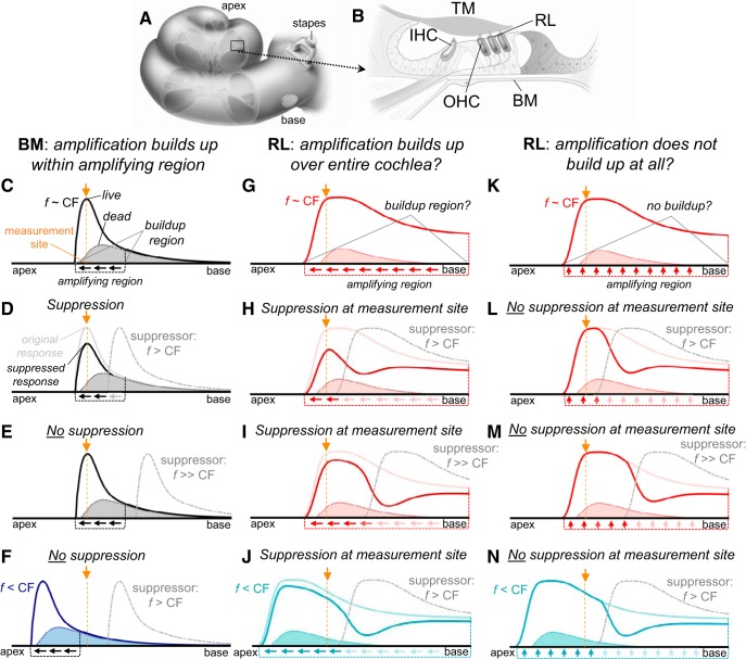
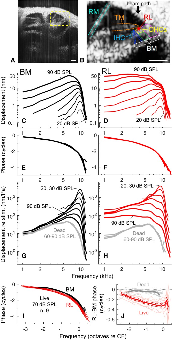
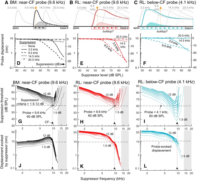
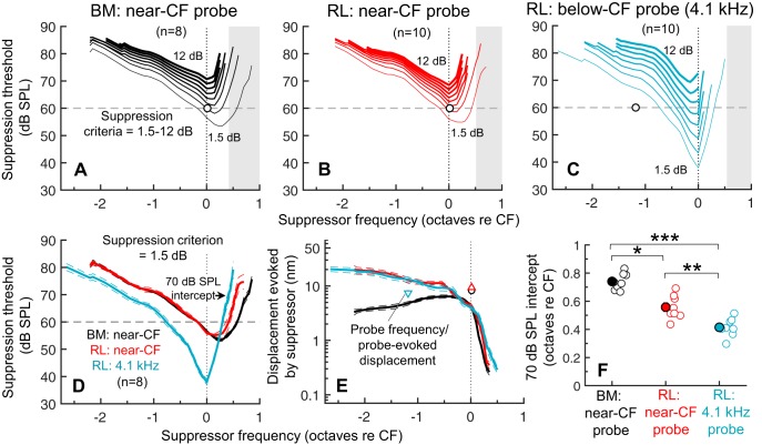
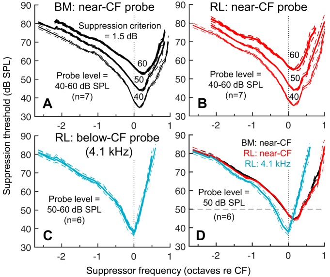
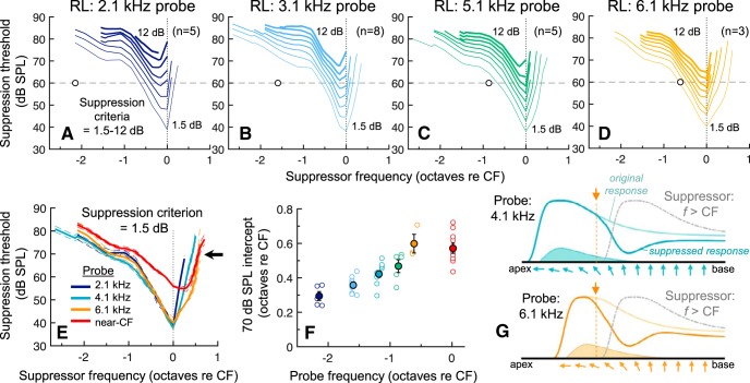
Mammalian hearing sensitivity and frequency selectivity depend on a mechanical amplification process mediated by outer hair cells (OHCs). OHCs are situated within the organ of Corti atop the basilar membrane (BM), which supports sound-evoked traveling waves. It is well established that OHCs generate force to selectively amplify BM traveling waves where they peak, and that amplification accumulates from one location to the next over this narrow cochlear region. However, recent measurements demonstrate that traveling waves along the apical surface of the organ of Corti, the reticular lamina (RL), are amplified over a much broader region. Whether OHC forces accumulate along the length of the RL traveling wave to provide a form of "global" cochlear amplification is unclear. Here we examined the spatial accumulation of RL amplification. In mice of either sex, we used tones to suppress amplification from different cochlear regions and examined the effect on RL vibrations near and far from the traveling-wave peak. We found that although OHC forces amplify the entire RL traveling wave, amplification only accumulates near the peak, over the same region where BM motion is amplified. This contradicts the notion that RL motion is involved in a global amplification mechanism and reveals that the mechanical properties of the BM and organ of Corti tune how OHC forces accumulate spatially. Restricting the spatial buildup of amplification enhances frequency selectivity by sharpening the peaks of cochlear traveling waves and constrains the number of OHCs responsible for mechanical sensitivity at each location.SIGNIFICANCE STATEMENT Outer hair cells generate force to amplify traveling waves within the mammalian cochlea. This force generation is critical to the ability to detect and discriminate sounds. Nevertheless, how these forces couple to the motions of the surrounding structures and integrate along the cochlear length remains poorly understood. Here we demonstrate that outer hair cell-generated forces amplify traveling-wave motion on the organ of Corti throughout the wave's extent, but that these forces only accumulate longitudinally over a region near the wave's peak. The longitudinal coupling of outer hair cell-generated forces is therefore spatially tuned, likely by the mechanical properties of the basilar membrane and organ of Corti. Our findings provide new insight into the mechanical processes that underlie sensitive hearing.

Keywords: basilar membrane; cochlear amplification; reticular lamina; traveling wave.

Figure 1.

Assessing the spatial buildup of amplification in the mouse cochlea using suppression. A, Diagram indicating the approximate location where we measured vibrations in the apical turn of the mouse cochlea. B, Cross-sectional diagram of the cochlear partition. The RL forms the apical surface of the OHCs and IHCs, which are coupled to the BM by various supporting cells. The overlying tectorial membrane (TM) is connected to the RL via the tallest row of OHC stereocilia. C, Diagram illustrating the spatial envelope of BM displacement along the length of the uncoiled cochlea. The response is shown for a stimulus frequency (f) near the CF (∼9 kHz) of our measurement site (orange dashed line) in an active, live cochlea (solid line) and a passive, dead one (dotted line/shaded region). BM responses are amplified in the region where live and dead responses diverge (dashed bracket) and amplification builds up over this region (indicated by apically-pointing arrows). D–F, Known effects of suppressor tones on BM responses to near-CF (D, E) and below-CF (F) tones. Near-CF responses are reduced by above-CF suppressor tones that excite the amplifying/buildup region (gray line, with f > CF; D) but not by suppressor tones that only excite more basal regions (with f ≫ CF; E). Below-CF responses are not reduced because there is no amplification to suppress at our measurement site (F). G, Envelope of the RL response to a near-CF tone in a live and dead cochlea, illustrating that RL motion is amplified throughout the traveling wave. Apically-pointing arrows indicate the hypothetical scenario in which amplification builds up throughout the amplifying region. H–J, Predictions for the suppression of RL responses if amplification builds up throughout the amplifying region. At our measurement site, RL responses to both near-CF (H, I) or below-CF (J) tones should be reduced by suppressors that excite any portion of the amplifying region, including those that excite regions far basal to the peak. K–N, Diagrams illustrating the alternate scenario in which amplification of the RL traveling wave does not build up at all (K). RL motion at any given location would therefore only be amplified by local OHC-generated forces (vertically-oriented arrows indicate local amplification). At our measurement site, RL responses to near-CF (L, M) or below-CF (N) tones should not be reduced by suppressor tones that do not excite this location.

Figure 2.

Single-tone responses of the BM and RL. A, Cross-sectional image of a mouse cochlea obtained in vivo with VOCTV. The measurement location in the apical turn is highlighted. Scale bar, 100 μm. B, Magnification of highlighted region from image in A with the locations of the BM, TM, Reissner's membrane (RM), and various cellular regions within the organ of Corti outlined. Outlined but not labeled are the pillar cells (in blue), which bound the tunnel of Corti; the Deiters' cells (in green), which support the OHCs; and the lateral supporting cell region (in magenta), which include Hensen's, Claudius', and Boettcher's cells. Stars indicate locations on the BM and RL where vibrations were measured. Scale bar, 100 μm. C, D, Sound-evoked displacements of the BM (C) and RL (D) obtained from a representative mouse at a location with a CF of 9 kHz. Displacement magnitudes are plotted as a function of the stimulus tone frequency (1–15 kHz in 0.5 kHz steps) for different stimulus levels (20–90 dB SPL, 10 dB steps). Curves for the lowest and highest stimulus levels are labeled. For clarity, displacements were smoothed across frequency with a three-point moving average. E, F, Phase of BM (E) and RL (F) displacements as a function of frequency. Curves for different stimulus levels largely overlap at the scale shown. Increasing phase lags with increasing stimulus frequency indicate traveling-wave propagation. G, H, Displacements of the BM (G) and RL (H) normalized to the evoking stimulus pressure in Pascals, revealing frequency- and level-dependent response nonlinearities. After death, BM and RL responses near the CF were dramatically reduced and nonlinearities were eliminated (overlapping gray curves were obtained for 60–90 dB SPL tones). RL responses below the CF were also reduced postmortem at all stimulus levels. I, Phase of BM and RL responses to 70 dB SPL tones for all live mice in which single-tone responses were obtained with sufficient frequency resolution at this stimulus level. Response phases were consistent across preparations, and reveal that RL motion progressively lagged BM motion with increasing stimulus frequency. The frequency axis is expressed in octaves relative to the CF to facilitate comparison across mice. J, The difference between the BM and RL response phases shown in I, as well as the RL–BM phase difference in the same mice after death, demonstrating that it was physiologically vulnerable. Individual and average data are shown with thin and thick lines, respectively (dashed lines indicate ±SEM). Individual data falling below the measurement noise floor are not shown. Average values are only shown for frequencies where data from at least five mice exceeded the noise floor.

Figure 3.

Suppression of responses to near-CF and below-CF probe tones. A–C, Diagrams illustrating the waves elicited by a probe tone fixed at a frequency near the CF of the measurement site (here 9.5 kHz) for the BM (A) and RL (B), or at a below-CF frequency for the RL (C). The waves elicited by suppressor tones at different frequencies are shown in gray. D, E, Representative BM (D) and RL (E) displacements evoked by a near-CF probe tone (9.6 kHz, 60 dB SPL) in the absence (thin, solid line) or presence of suppressor tones at frequencies below, at, or above the CF (see legend), plotted as a function of suppressor level. Right axes indicate the amount of suppression in dB relative to the unsuppressed probe response. For clarity, the unsuppressed probe response was averaged across all measurement conditions. Responses in the presence of each suppressor (in nm) were rescaled appropriately using the amount of suppression (in dB) observed in each condition. F, RL displacements for a below-CF (4.1 kHz) probe tone in the absence and presence of the same suppressor tone frequencies. The probe response was relatively insensitive to above-CF suppressor tones, indicating that amplification of the response did not build up from locations basal to the measurement site. G–I, Suppressor tone levels required to achieve fixed amounts of suppression, ranging from 1.5–12 dB in 1.5 dB steps, as a function of suppressor tone frequency (data are from the same preparation as in D–F). The CF is indicated by the triangle/dotted vertical line; dashed horizontal line and circle indicate the probe frequency and level. Gray shaded regions indicate the range of suppressor frequencies for which the suppressor evoked no displacement above the measurement noise floor (∼0.1 nm). J–L, Displacements elicited by the suppressor tone at the threshold for each suppression criterion shown in G–I. Suppressor-evoked displacements falling below the measurement noise floor are not shown. Dashed horizontal line indicates the unsuppressed response to the probe tone.

Figure 4.

Average suppression thresholds for BM and RL responses to near-CF probes and RL responses to below-CF probes. A–C, Average suppressor levels required to suppress BM (A) and RL (B) responses to near-CF probes, and RL responses to a 4.1 kHz probe (C) by 1.5–12 dB. Because of the different CFs across preparations (9 or 9.5 kHz), suppressor frequencies are expressed in octaves relative to the CF, and suppression thresholds were interpolated to facilitate averaging. Circles/dashed horizontal lines indicate the probe frequency/level; dotted vertical lines highlight the CF position. Shaded gray area indicates the range of suppressor frequencies for which the displacement evoked by the suppressor was below the measurement noise floor (∼0.1 nm). Error bars not shown for clarity. D, Comparison of average suppression thresholds (criterion = 1.5 dB) from mice in which all three measurement conditions were obtained. Data are shown only at frequencies where suppression thresholds were measurable in at least five mice. Dashed lines indicate ±SEM. The 70 dB SPL intercept used to calculate the spatial extent of the buildup region is indicated. E, Average displacements evoked by the suppressor tone that reduced each probe response by 1.5 dB. Symbols indicate the frequencies and average displacements elicited by the near-CF and below-CF probe tones when presented alone (error bars are smaller than the symbols). F, Comparison of 70 dB SPL intercepts for 1.5 dB of suppression. Suppression of BM and RL responses to near-CF probes extended to significantly higher suppressor frequencies compared with the suppression of RL responses to a 4.1 kHz probe. BM responses to near-CF probes were also suppressed by significantly higher suppressor frequencies than were RL responses to near-CF probes. Asterisks indicate statistical significance. *p < 0.05, **p < 0.005, ***p < 0.0005, repeated-measures ANOVA followed by post hoc comparisons with Bonferroni corrections.

Figure 5.

Suppression extends to higher suppressor frequencies with decreasing probe level for near-CF, but not below-CF, probes. A, B, Average suppression thresholds (criterion = 1.5 dB) for BM (A) and RL (B) responses to near-CF probe tones presented at levels of 40, 50, and 60 dB SPL. With decreasing probe level, suppression was observed at lower suppressor levels and higher suppressor frequencies, indicating a broadening of the buildup region. Averages include data from mice in which suppression was characterized for all three probe levels, and are shown only at frequencies where suppression criteria were met in at least five mice. C, Average suppression thresholds (criterion = 1.5 dB) for RL responses to a 4.1 kHz probe presented at 50 and 60 dB SPL. Suppression thresholds for the two probe levels were highly similar. Average data inclusion/plotting criteria are as described above. D, Comparison of average suppression thresholds for 50 dB SPL probes. Dashed horizontal line indicates the probe level. For all curves in A–D, dashed lines indicate ±SEM. Dotted vertical lines highlight the CF position.

Figure 6.

Suppression of RL responses to different below-CF probes reveals a gradual transition between the region of the RL traveling wave where amplification builds up and where it is primarily local. A–D, Average suppression thresholds for RL responses to probe frequencies of 2.1, 3.1, 5.1, and 6.1 kHz (A–D, respectively) for a probe level of 60 dB SPL. Circles/dashed horizontal lines indicate the probe frequency and level; dotted vertical lines highlight the CF position. Averaged data are only shown at frequencies where the suppression criterion was met and displacements were above the noise floor in at least five mice (when n = 8), four mice (when n = 5), or in three mice (when n = 3). Error bars not shown for clarity. E, Comparison of average suppression thresholds (criterion = 1.5 dB) for RL responses to 2.1, 4.1, and 6.1 kHz probes, as well as a near-CF probe. Dashed lines indicate ±SEM. F, Comparison of the 70 dB SPL intercept of the suppression threshold curves (indicated by arrow in E) for all probe frequencies. With decreasing probe frequency, above-CF suppressor tones became progressively less effective at suppressing the probe response, indicating that the buildup region became increasingly narrow. Individual/average data are shown with open/filled symbols. Error bars indicate ±SEM. G, Diagram illustrating that the data suggest a smooth transition between the region of the traveling wave where amplification builds up (apically-pointing arrows), and where amplification is primarily local (vertical arrows). The position of our measurement site (orange arrows/vertical dashed lines) in this transition region explains the increased effectiveness of an above-CF suppressor tone (dashed gray lines) in suppressing the response to a 6.1 kHz versus a 4.1 kHz probe tone. The passive response to each probe tone is also shown (dotted curves/shaded regions).

References

1. Ashmore J, Avan P, Brownell WE, Dallos P, Dierkes K, Fettiplace R, Grosh K, Hackney CM, Hudspeth AJ, Jülicher F, Lindner B, Martin P, Meaud J, Petit C, Santos-Sacchi JR, Sacchi JR, Canlon B (2010) The remarkable cochlear amplifier. Hear Res 266:1–17. 10.1016/j.heares.2010.05.001 - DOI - PMC - PubMed
1. Békésy von G. (1960) Experiments in hearing. New York: McGraw-Hill.
1. Charaziak KK, Siegel JH (2015) Tuning of SFOAEs evoked by low-frequency tones is not compatible with localized emission generation. J Assoc Res Otolaryngol 16:317–329. 10.1007/s10162-015-0513-0 - DOI - PMC - PubMed
1. Cheatham MA, Dallos P (1982) Two-tone interactions in the cochlear microphonic. Hear Res 8:29–48. 10.1016/0378-5955(82)90032-6 - DOI - PubMed
1. Cody AR. (1992) Acoustic lesions in the mammalian cochlea: implications for the spatial distribution of the “active process”. Hear Res 62:166–172. 10.1016/0378-5955(92)90182-M - DOI - PubMed
Publication types
LinkOut - more resources