. 2019 Jan 24;9(1):456.
doi: 10.1038/s41598-018-36861-8.

Speed-Selectivity in Retinal Ganglion Cells is Sharpened by Broad Spatial Frequency, Naturalistic Stimuli

Affiliations

Speed-Selectivity in Retinal Ganglion Cells is Sharpened by Broad Spatial Frequency, Naturalistic Stimuli

César R Ravello et al. Sci Rep. .

Abstract

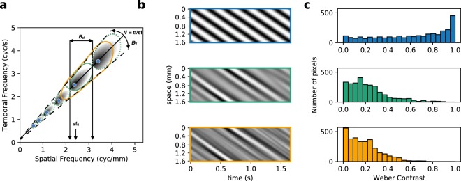
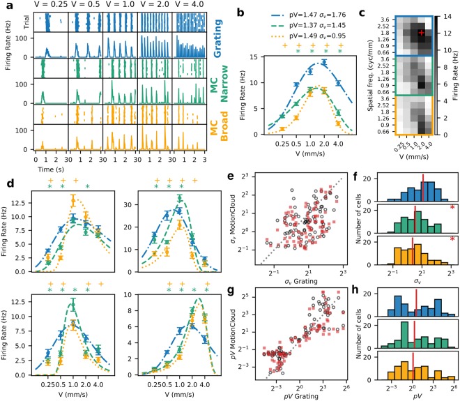
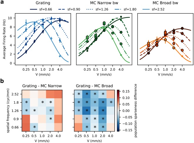
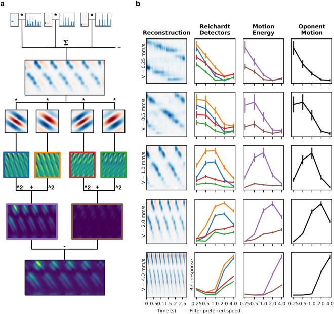
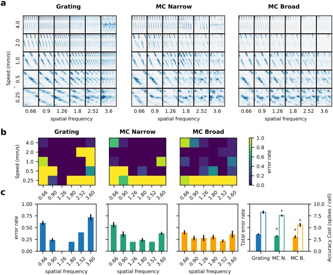
Motion detection represents one of the critical tasks of the visual system and has motivated a large body of research. However, it remains unclear precisely why the response of retinal ganglion cells (RGCs) to simple artificial stimuli does not predict their response to complex, naturalistic stimuli. To explore this topic, we use Motion Clouds (MC), which are synthetic textures that preserve properties of natural images and are merely parameterized, in particular by modulating the spatiotemporal spectrum complexity of the stimulus by adjusting the frequency bandwidths. By stimulating the retina of the diurnal rodent, Octodon degus with MC we show that the RGCs respond to increasingly complex stimuli by narrowing their adjustment curves in response to movement. At the level of the population, complex stimuli produce a sparser code while preserving movement information; therefore, the stimuli are encoded more efficiently. Interestingly, these properties were observed throughout different populations of RGCs. Thus, our results reveal that the response at the level of RGCs is modulated by the naturalness of the stimulus - in particular for motion - which suggests that the tuning to the statistics of natural images already emerges at the level of the retina.


Conflict of interest statement

The authors declare no competing interests.

Figures

Figure 1
Figure 1
Motion Cloud (MC) stimuli are characterized by the parameters of their spatio-temporal spectral envelope. (a) Bi-dimensional representation of the spatio-temporal frequency space. Points along the continuous line correspond to simple drifting grating stimuli moving at a given speed but with different spatial frequencies (blue dots). MC stimuli have their spectral energy distributed in an “ellipse” warped along a given speed plane. Interestingly, these can be parameterized with the same mean spatial (sf0) frequency and speed (V) as gratings, but with different levels of spatial frequency bandwidths (defined by the parameter Bsf, with Bsf = 0 for the grating) which will define the level of complexity of the sequence. The green ellipse represents a narrow bandwidth stimulus and the orange ellipse a broader bandwidth stimulus. (b) Examples of stimuli at different complexity levels. For simplicity, we plot the light intensity along a single row of the image (vertical axis) for the whole duration of the stimulation (horizontal axis). We show the drifting grating (top panel), which is constituted by a single spatial and temporal frequency (and thus a single speed, seen as the slope in this view), and the MCs (middle and lower panels), which have the same speed and central spatial frequency but with a narrow or wide bandwidth in spatial frequency space. (c) Contrast distribution of the stimuli. The three types of stimuli were built to have the same Michelson contrast, but their contrast distribution is different. By construction, sinusoidal gratings have a higher proportion of brightest and darkest pixels, while the rest of the values have uniform representation; on the other hand, MCs have a large proportion of pixels with intermediate luminance, with extreme values being rare, resulting in images where low contrast is more frequent than high contrast, as is the case of natural images.
Figure 2
Figure 2
Experimental multielectrode recording setup. (a) Schematic view of the retina over a Multielectrode Array, while light stimulation is projected from below. (b) Each blue line represents a voltage signal from an electrode, and the red dots indicate detected peaks. (c) The signal of each electrode is reconstructed by iteratively adding different templates. Each color represents a different template, indicating spikes coming from different cells. Each spike can be detected by many neighboring electrodes, but only one will be assigned to a single unit. (d) The raster plot indicates the times at which each RGC fired an action potential. (e) Spike Triggered Average (STA) of a representative cell, computed from the response to checkerboard stimulus. Each panel shows the average image at the corresponding frame before the spiking of the cell (time zero). Blue pixels represent points with negative contrast, while red represent those with positive contrast. The black bar is 0.2 mm long. (f) Spatial component of the STAs of all the RGCs recorded from a retinal patch, after discarding non-valid units (see Methods for details). Each ellipse corresponds to a 2-D Gaussian fit at 1 s.d. The background shows the frame from (e) of maximum response and the red ellipse its fit, while the blue ellipses show the fit for the rest of the cells. (g) Distribution of RF sizes from a retinal patch, measured as the radius of a circle with the same area as the ellipse fit. (h) Temporal components of the STA of the cells shown in (g). The crosses mark the STA of the cell shown in (e).
Figure 3
Figure 3
Response to variations in speed and spatial frequency of the drifting grating stimulus. (a) Raster and PSTHs of the response of a representative RGC at each speed and spatial frequency tested. (b) The response to speed at each spatial frequency sf was fitted to a skewed Gaussian. Each point is the average of the PSTH, with the error bars showing SEM. (c) All cells that had a good fit (χ2 < 0.05) at every sf were classified as speed responsive cells. For all these cells, the preferred speed at each spatial frequency is determined from the fits to their distribution. Vertical red lines show the median of the distribution for each condition.
Figure 4
Figure 4
Speed responsive retinal ganglion cells. (a) Left: Map of the RGCs RF present in the experiment analyzed. RF of speed responsive (SR) RGCs (see text) are represented in color. Right: Temporal profiles of the receptive field center of SR (in red) and Non-SR (in black) cells. (b) Sample of a temporal profile showing the parameters extracted to compare SR versus Non-SR cells, which in this case are zero-cross and peak-time. (c) Histograms representing the distribution of the zero-cross (left) and peak-time (right) parameters in the SR and Non-SR population cells. We only observe significant differences for the zero-cross parameter (D = 0.22 p = 0.026 versus D = 0.11 p = 0.65 for the peak-time parameter, Kolmogorov-Smirnov test).
Figure 5
Figure 5
A large part of the population of observed RGCs narrow down their tuning selectivity with higher complexity stimuli. (a) Raster and PSTHs of the response of a representative cell for each type of stimulus and to the different speeds (in mms−1) at its preferred sf0. (b) The change in tuning is evident when plotting the average response and its fit. Each point is the average of the PSTH, with the error bars showing s.d. The asterisks (for the Narrow bandwidth) and crosses (Broad bandwidth) mark the speeds at which the response to the MC is significantly different from the response to the grating (p < 0.05 Wilcoxon signed-rank test). The narrowing of the curve can be quantified by the decrease in the σv parameter, which in the case of this cell decreased with the complexity of the stimulus. (c) Spatiotemporal tuning of the cell for the different types of stimuli. The intensity at each square denotes the average firing rate for the corresponding stimulus parameters. The red cross indicates the point of maximum response, and corresponds to the spatial frequency plotted in panels a and b. (d) Additional examples of cells with narrower tuning for the naturalistic stimulus. (e) Joint distribution of speed tuning bandwidth coefficients σv of each Speed Responsive Cell. Empty circles show the relationship of grating against narrow bandwidth MC, filled squares show grating against broad bandwidth MC. In both conditions most of the points fall below the line of identity. (f) Histograms show the distribution of σv. Vertical red lines show the median of each distribution. The distribution for gratings is centered, while the distributions for both types of MC are skewed towards lower values with a significant difference (T = 1009 p = 0.00216 for grating vs. narrow bw. MC, T = 843 p = 0.00012 for the broad bw. MC, Wilcoxon signed-rank test). (g,h) same as (e,f) but for the preferred speed (peak of the fitted curve) with a less significant difference (T = 1159 p = 0.018 for grating vs. narrow bw. MC, T = 1632 p = 0.893 for the broad bw. MC, Wilcoxon signed-rank test).
Figure 6
Figure 6
Naturalistic stimuli and sparse code. (a) Changes in Tuning to Speed at the population level. The dots show the average response across trials for the whole population of Speed Responsive RGCs for each combination of speed and spatial frequency used; the lighter shades show increasing spatial frequency, the error bars show standard deviation. The encircled dots indicate all the conditions for which the response is significantly smaller than the response to the grating stimulus (p < 0.05 Wilcoxon signed-rank test). The response to speeds for each spatial frequency was fitted to an skewed Gaussian. As expected, at higher spatial frequencies the preferred speed shifts towards lower values, together with a decrease in maximum response, however, this decrease becomes more pronounced when the complexity of the stimulus increases, to the point where the response to lower speeds becomes very similar for different spatial frequencies (no significant difference at speeds 0.25 and 0.5 mms (p > 0.05 Wilcoxon signed-rank test). (b) Sparseness in the code, calculated as population sparseness (eq. 5), is a measure of how many RGCs are responding and their relative level of activity. The 2-D plots show the difference in average sparseness between grating and MC for each condition tested. In general, it is higher for the extreme parameters, however, for the more complex stimulus, the area of high sparseness is larger. The asterisks indicate the conditions for which the sparseness is higher compared to that obtained using grating stimulus (Wilcoxon signed-rank test, p < 0.05).
Figure 7
Figure 7
Reconstruction and decoding of motion stimuli. (a) The scheme shows the the stages of the motion decoding algorithm and the results of each step. (b) The leftmost column of each plot shows the reconstruction of the moving stimulus at different speeds, at a spatial frequency of 0.9cycles/mm. From the population response, the stimulus is reconstructed by convolution of the spike train with the RF of each RGC. The reconstructions are dominated by negative contrasts, due to the low number of ON type cells and their relatively low response. The mostly white row in each reconstruction corresponds to an area of the patch with no recorded units. The following columns show the response at each stage of decoding, for each corresponding reconstruction, averaged across trials. Vertical bars show s.d. The first stage is the response of each of the four filters that constitute the Reichardt detectors, the following column shows the Motion Energy in each direction and the rightmost column is the difference between the two. The color of each line corresponds to the respective panel of (a); For each reconstruction the decoding is considered correct if, in the final stage, the preferred speed of the most activated filter matches the stimulus speed.
Figure 8
Figure 8
Precision of the estimation of stimulus speed. (a) Reconstruction of every motion stimulus tested. The representation is the same as in Fig. 7. For the three types of stimulus, the motion traces (and their slopes) are easily seen for all conditions, except at the lower speeds and higher spatial frequencies, which is consistent with lower responses under those conditions (Fig. 6). (b) Error rate in the decoding of the speed estimation (number of times that the algorithm estimated the correct speed over the total number of trials). The 2-D plots show the error rate at each spatial frequency and speed, for each type of stimulus. (c) Error rate for each spatial frequency and total error rate. Error lines show standard deviation between trials. Bars with no error mean that speed decoding was successfully performed between stimulus repetitions, for a given condition. In the rightmost plot, solid columns show total error rate and open bars show the Accuracy cost. Accuracy cost is computed as the success rate multiplied by the average firing (total number of spikes/number of cells); asterisks indicate significant difference with respect to the Grating (p < 0.05 Wilcoxon signed-rank test).

Similar articles

Cited by

References

    1. Barlow HB, Hill RM, Levick WR. Retinal ganglion cells responding selectively to direction and speed if image motion in the rabbit. The Journal of Physiology. 1964;173:377–407. doi: 10.1113/jphysiol.1964.sp007463. - DOI - PMC - PubMed
    1. Olveczky BP, Baccus SA, Meister M. Retinal adaptation to object motion. Neuron. 2007;56:689–700. doi: 10.1016/j.neuron.2007.09.030. - DOI - PMC - PubMed
    1. Vaney, D. I., Sivyer, B. & Taylor, W. R. Direction selectivity in the retina: symmetry and asymmetry in structure and function. Nature Reviews Neuroscience 1–15 (2012). - PubMed
    1. Burr D, Thompson P. Motion psychophysics: 1985-2010. Vision Research. 2011;51:1431–1456. doi: 10.1016/j.visres.2011.02.008. - DOI - PubMed
    1. Simoncelli EP, Olshausen BA. Natural image statistics and neural representation. Annual Review of Neuroscience. 2001;24:1193–1216. doi: 10.1146/annurev.neuro.24.1.1193. - DOI - PubMed

Publication types